Power Query Parameters: 3 methods + 1 simple example

As Power Query records transformation steps, it includes many hardcoded values within the M code. For example, if we filter a column to select all values greater than 50, the 50 is a hardcoded value in the M code. For something more dynamic, that we can easily change, we use Power Query parameters.

Obviously, we could edit the query each time we want to use it. However, this would be very time-consuming (and become very annoying, very quickly). So instead, parameters are the best way to make our queries flexible for different outputs.

Table of Contents

• What is a Power Query parameter?
• Scenario
• Create the query
• Apply transformations
• Create the parameters
• Create the Text parameter
• Create the Date parameter
• Insert the parameters into the query
• Using the parameters
• Other types of parameters
• Manage parameters
• Static values
• Notes
• Formula Firewall & Privacy
• How to select all
• Wrap-up

The download contains the source data and the completed solution. In this post, we work through all the steps from start to finish to demonstrate how to build the complete solution. So, open up the 0103 Power Query Parameters.xlsx workbook, and let’s get going.

Watch the video

Watch the video on YouTube.

What is a Power Query parameter?

The term “Parameter” may seem a bit confusing. We use the term variable when writing VBA, or in Excel, we might use the terms conditions, criteria, or arguments. Effectively, these all describe the same thing. Parameters, variables, conditions, criteria, and arguments are all values we change to obtain a different output. Microsoft decided to use the term Parameter when designing Power Query.

There are many ways to create parameters. Initially, this post focuses on creating parameters from cell values. As Excel users, these will be the most useful for our needs. Later in the post, we consider other methods to give you a complete picture. Then you can choose the best approach for your scenario.

Technically, using values from cells cannot be called a parameter. This is because, in Power Query, parameters have a particular method of creation. However, for our purposes, cell values can operate like parameters; we will use them like parameters; so let’s just call them “unofficial” parameters. There is more on “official” parameters later in the post.

Scenario

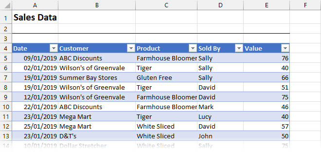
In our example scenario, we want to filter the data for a specific date and employee name based on cell values. So, each time we refresh the data, Power Query reads the current cell values and applies them as parameters in the query.

This is the example data we are using:

Create the query

The first step is to create a query as normal.

Select a cell from the source table and click Data > From Table/Range from the ribbon.

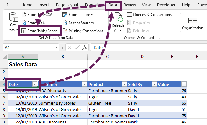
The Power Query editor opens with the data.

Apply transformations

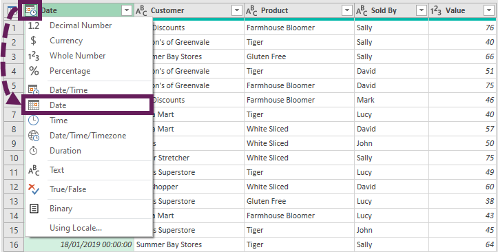
Let’s make the following transformations

Click on the Date and Time icon next to the Date header, and select Date from the data type menu.

Select the Date column header, then click Transform > Date > Month > End Of Month

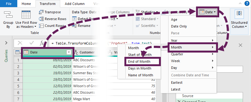
All values in the Date column are now month-end dates.

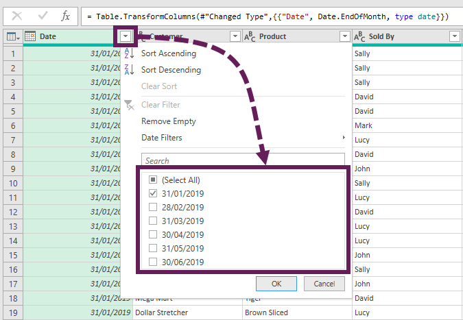
Filter the Date column only to include 31 January 2019. Please note, the date format may appear different depending on your location settings.

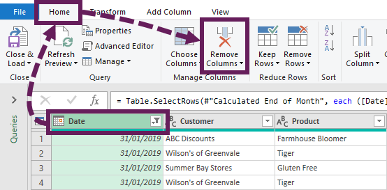
Ensure the Date column is still selected, then click Home > Remove Columns

The transformations required for the Sold By column are similar to those above.

On the Sold By column, click on the filter icon and ensure only David is selected.

With the Sold By column still selected, click Home > Remove Columns.

That’s enough transformations for now. Name the query SalesData, then click Home > Close and Load to load the data into an Excel Table on the worksheet.

The Table should look like this,

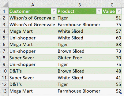
From the source data, we created a table showing David’s products in January 2019. But what if we want the products sold by Sally in March 2019, or Mark in February 2019? This is where the parameters come in. 

In the next section, we create parameters to change the name and date dynamically.

Create the parameters

As noted above, initially, we are focusing on cell-based parameters. In these scenarios, a parameter is just a standard query in which we drill down into the value of a single cell. This parameter query is not loaded back into the worksheet; it is purely used as a placeholder in the M code of another query. As a result, all parameter queries are loaded as a connection only.

In this example, we are using an Excel Table as the source for parameters, but it could equally be a named range, CSV, SharePoint list, or any other data source we can get into Power Query.

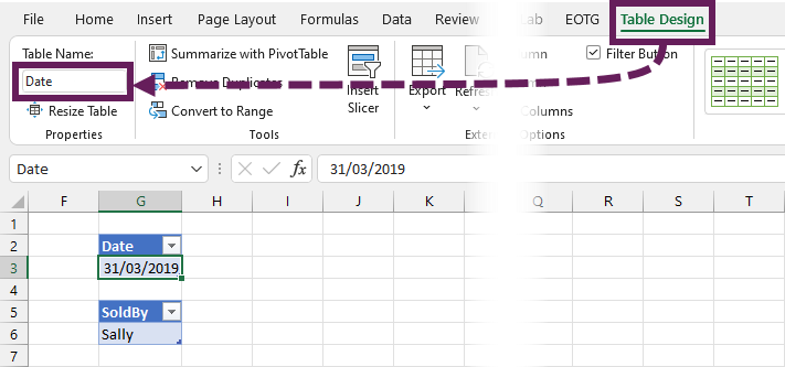
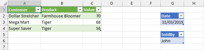
On the worksheet that contains the query output table, create two tables with single values in each.

Table 1

• Header: Date
• Value: 31 March 2019

Table 2

• Header: Sold By
• Value: Sally

After creating each Table, rename them, so they have meaningful names. The first Table I named Date, and the second SoldBy.

Create the Text parameter

First, let’s create the parameter to hold the name.

Select the cell in the SoldBy table and create a query by clicking Data > From Table/Range.

We need to pay close attention to the data type. The Sold By column in the original SalesData query was a text data type. The data type for this query must also be text. If necessary, change the data type to text.

Next, within Power Query, right-click on the value and select Drill Down from the menu.

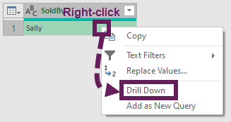
The window will change to a view we have not seen before, the Text Tools view.

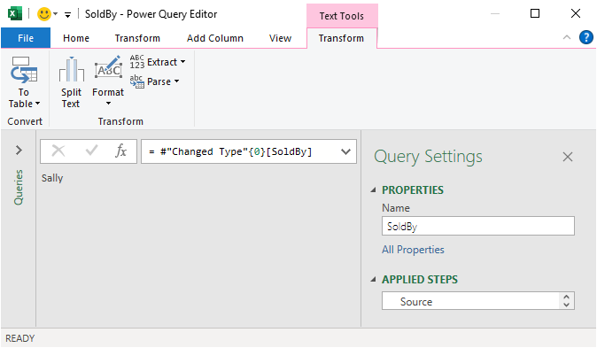
We don’t need the SoldBy query on our worksheet; therefore, we want to load it as a connection only. Click File > Close & Load To… (or Home > Close & Load (drop-down) > Close and Load To…).

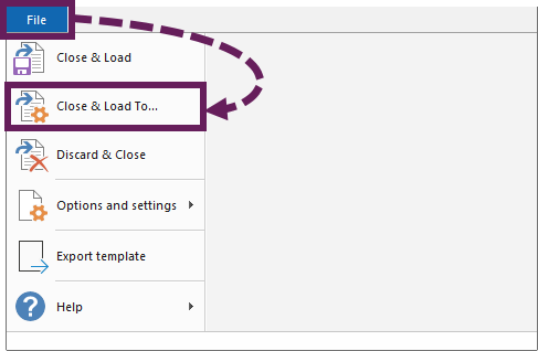
From the Import Data dialog box, select Only Create Connection, then click OK.

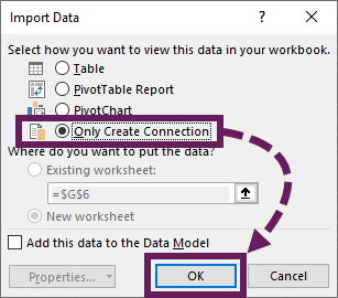
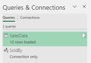
The Queries & Connection pane will now show two queries: the original query, SalesData, and the text parameter, SoldBy.

Create the Date parameter

OK, let’s repeat the same steps for the Date parameter. 

As noted above, parameters need to have the correct data type. In the original SalesData query, the Date column had a date type. Therefore, we need the parameter to have a date type too.

Load the Date table into Power Query. Then, click on the icon next to the Date header and select Date from the menu. This changes the column to a date data type.

Next, right-click on the value and click Drill Down. Rather than Text Tools, as we saw for the first parameter, this time it will be the DateTime Tools view.

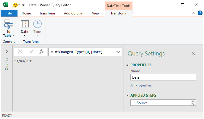
As before, click Close & Load To…

Then, in the Import Data dialog box, select Create Connection Only and click OK.

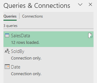
We should now have two parameters created, SoldBy as a text type and Date as a date type.

Insert the parameters into the query

We have created the parameters; we are now ready to use them. To do this, we will make simple M code changes. We could use the Advanced Editor or the Formula Bar for this. To keep things simple, we’ll use the Formula Bar.

Important: Be careful of your typing because M code is case-sensitive.

Open the original SalesData query.

If the Formula Bar is not visible, click View > Formula Bar from the ribbon.

Find the step where we hard-coded the value, David.

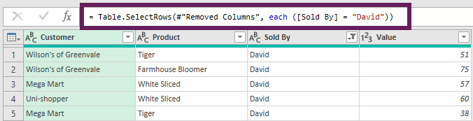
Replace “David” for the parameter SoldBy.

= Table.SelectRows(#"Removed Columns", each ([Sold By] = "David"))

Becomes:

= Table.SelectRows(#"Removed Columns", each ([Sold By] = SoldBy))

Next, let’s apply the Date parameter. Find the step where we hardcoded 31 January 2019 as the date.

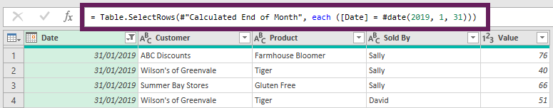
Replace #date(2019, 1, 31) for the parameter Date.

= Table.SelectRows(#"Changed Type1", each ([Date] = #date(2019, 1, 31)))

Becomes:

= Table.SelectRows(#"Changed Type1", each ([Date] = Date))

That’s all there is; we have applied the parameters. 

Click Home > Close & Load to load the changes into Excel.

Using the parameters

Once we are back in Excel, we can change the Date and Sold By table values, then click Data > Refresh All.

The query refreshes to show only the items we have requested.

Wow! Magic, eh!

We can use this method to set up any Power Query hardcoded value as a parameter. I find the most useful things to set up as parameters are:

• File paths to import external data files (check out this post for more details: Change Power Query source based on cell value)
• Period end dates for financial reports
• Names of business divisions or cost centers to create reports for specific areas only
• Any settings another user is likely to need to change

These are the type of scenarios we are most likely to face as Excel users.

Other types of parameters

Technically, what we have seen so far are not “parameters”. Parameters inside Power Query have special features. We have used queries linked to cells to behave like parameters. But they do not contain the special features.

Manage parameters

Official parameters have features which Power Query uses for advanced functionality (e.g., Custom functions or incremental refresh inside Power BI). However, we often don’t use these features, which is why we considered cell based values first.

Let’s create the parameters we used in our example.

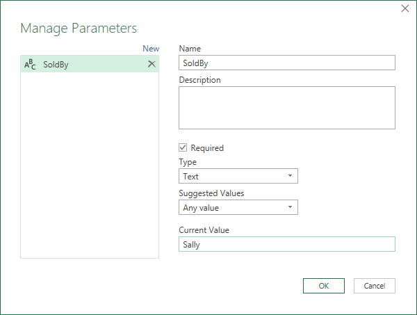
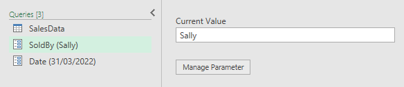
In Power Query, click Home > Manage Parameters to open the Manage Parameters dialog box.

Click New to create a new parameter, then enter the following details:

• Name: SoldBy
• Type: Text
• Current Value: Sally

Click OK to close the dialog box.

The details for the Date query are:

• Name: Date
• Type: Data
• Current Value: 31/03/2019 (this is a UK date format, use your local date format if you’re following along)

This method creates parameters we can change through Power Query’s user interface.

While these parameters have special purposes, they are used in the SalesData query in precisely the same way.

Static values

There is another way to create an “unofficial” parameter inside Power Query.

In the primary example above, we turned a regular query into an unofficial parameter by drilling down into a single value. We can use this approach with any data source. However, we can also use any query containing a single value.

Below is an example of a Blank Query where the value is entered directly into the formula bar.

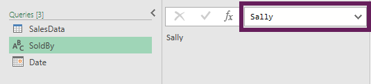
To use these simple parameters, we open Power Query and change the values as required.

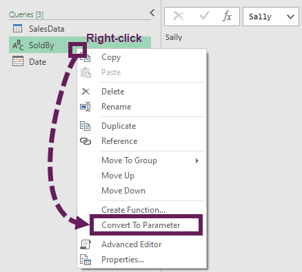
Even though these are single values queries, they can easily be converted to official parameters by right-clicking on the query and selecting Convert to Parameter from the menu.

Notes

Here are a few things to help you along the journey of implementing Power Query parameters

Formula Firewall & Privacy

If you start using Parameters to pass data between data different sources, you will likely encounter the Formula Firewall error and Privacy issues. For more information on this and how to resolve the problem, look at this post: https://www.thepoweruser.com/2019/03/12/data-privacy-and-the-formula-firewall/

How to select all

This method can work with multiple values, but I decided to keep things simple and not demonstrate it in this post.

If you want a switch to revert back to show all items, follow this post: Filter All in Power Query

Wrap-up

This post shows us how to create Power Query parameters in various forms. I believe the cell-linked parameters are the most valuable and flexible for Excel users. However, if we need more advanced functionality, we have also seen how to use Power Query’s built-in parameters functionality.

---

Read more posts in this series

1. Introduction to Power Query
2. Get data into Power Query – 5 common data sources
3. DataRefresh Power Query in Excel: 4 ways  &  advanced options
4. Use the Power Query editor to update queries
5. Get to know Power Query Close & Load options
6. Power Query Parameters: 3 methods
7. Common Power Query transformations (50+ powerful transformations explained)
8. Power Query Append: Quickly combine many queries into 1
9. Get data from folder in Power Query: combine files quickly
10. List files in a folder & subfolders with Power Query
11. How to get data from the Current Workbook with Power Query
12. How to unpivot in Excel using Power Query (3 ways)
13. Power Query: Lookup value in another table with merge
14. How to change source data location in Power Query (7 ways)
15. Power Query formulas (how to use them and pitfalls to avoid)
16. Power Query If statement: nested ifs & multiple conditions
17. How to use Power Query Group By to summarize data
18. How to use Power Query Custom Functions
19. Power Query – Common Errors & How to Fix Them
20. Power Query – Tips and Tricks

---

What next?

Discover how you can automate your work with our Excel courses and tools.

The Excel Academy