Power Query: Lookup value in another table with merge

Looking up data from a table or worksheet is probably the most common activity undertaken by Excel users to create reports. Learning to use VLOOKUP for many is their first taste of Excel’s power. But what about when using Power Query? There isn’t a VLOOKUP function, so how can we lookup a value from another table with Power Query? Well… in Power Query, we use the merge transformation.

The merge transformation in Power Query enables us to join tables together using a common reference. Therefore, it can do more than just look up values from another table. By the end of this post, I am sure you will appreciate the additional power that merges gives us.

Table of Contents

• Overview
• Scenario
• Load the data into Power Query
• Lookup value in another table with an exact match
• Types of joins
• Outer Joins
• Inner Join
• Anti Joins
• Lookup value from another table with an approximate match
• Multiple matches
• Multiple Criteria Lookup
• Fuzzy Match Lookup
• Conclusion

Watch the video

Watch on YouTube

Overview

Effectively there are three types of lookup, an exact match, an approximate match, and a fuzzy match.

• Exact match: The most common and require the lookup value to be identical.
• Approximate match: Finds the value above (or below) the lookup value.
• Fuzzy match: Finds values based on how similar they are to other values using a pattern-matching algorithm.

Power Query can do all of these lookup types, though, in this post, we focus primarily on the first two.

Scenario

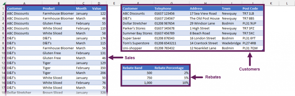
In the 0111 Lookup Data.xlsx example file there are three tables:

• Sales: Contains monthly sales data
• Customers: Contains customer contact information
• Rebates: Details the discount given to customers for buying over specific values.

To illustrate how we lookup a value in another table in Power Query we will create two reports.

Total Sales by Town (lookup with an exact match)
The Sales values and Town of each customer are in separate tables. Therefore, to calculate the total sales for each town, we need to use the Merge transformation to join the tables together.

Total Rebate by Customer (lookup with an approximate match)
To get each customer’s rebate, we need to perform an approximate match. We don’t necessarily want to match the exact value, but to find the band in which the sales value falls. We still use the Merge function to look up the value, but we will need a few more transformations to get the correct result.

Load the data into Power Query

Start by loading the three example tables into Power Query.

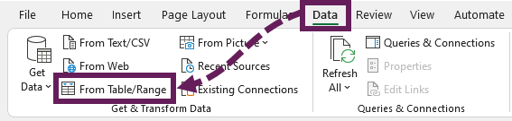
Click on any cell in the Sales table, then click Data > From Table / Range from the Excel ribbon.

The Power Query Editor loads.

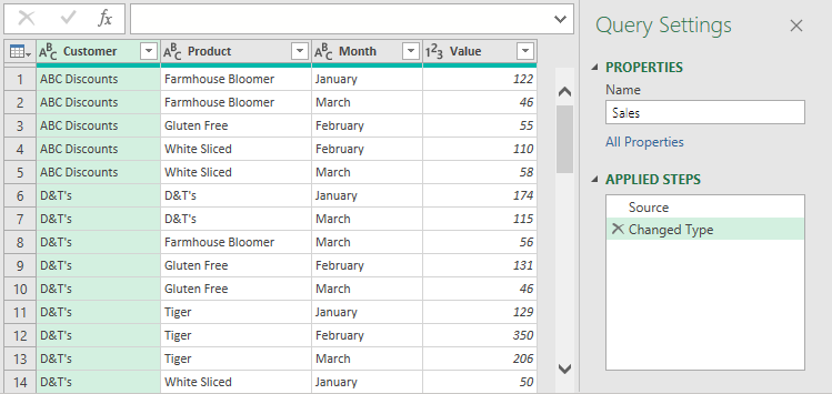
The example tables are purposefully set up so they require minimal transformations, but it is rarely this simple in the real world. In this example, the default data types applied by Excel are OK to use.

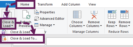
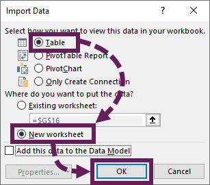
For our example, we do not need to load the data into the worksheet. Instead, we load the data as a connection. From the Power Query ribbon, click Home > Close & Load To…

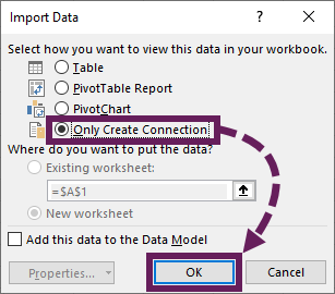
Select Only Create Connection from the Import Data window, then click OK.

Repeat this action with the Customers and Rebates tables in the example file. The only difference is to apply a Percentage data type to the Rebate Percentage column of the Rebates query.

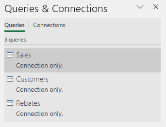
In Excel, open the Queries & Connections pane (Click Data> Queries & Connections if it is not visible), and the three queries should be listed.

Now we are ready to start using the Merge feature 😀

Lookup value in another table with an exact match

To illustrate an exact match, we will create a report of total sales by town.

Let’s get back into the Power Query editor by double-clicking on the Sales query within the Queries and Connections pane.

In the Power Query editor select Home > Merge Queries (drop-down).

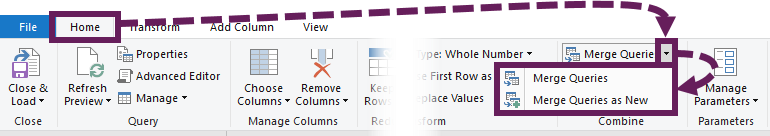
There are two options here, Merge Queries and Merge Queries as New. The difference between them is whether the transformation creates a new query, or adds the merged table as a transformation step within an existing query.

For ease, we will use a new query. So, select the Merge Queries as New option.

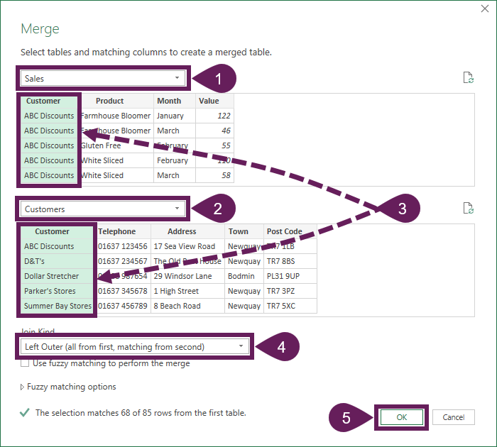
The Merge window opens. A lot is going on here:

1. Select the first query to be used – for our example, it is the Sales query.
2. Select the second query to be used – in our example, it is the Customer query.
3. Select the Customers column from both tables, as they are the columns with the common reference.
4. The Join Kind provides six different types of merges. For our first scenario, we need the Left Outer join.
5. Click OK.

Power Query merges the queries, by looking up from the first table into the second table.

There are 6 join types available; look at the section below to find out about the other join types.

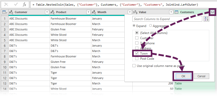
A new query is created, probably called Merge1. The first query selected in the Merge window is displayed, with an additional column containing the table of the second query.

Click on the expand table icon in the header of the Customers column. We only need the Town column selected, then click OK.

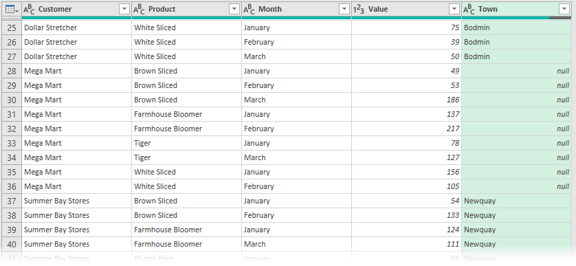
The selected join included all items from the Sales table and the matching items from the Customers table—any items without a match display null. For example, the customer Mega Mart exists in the Sales query but not the Customers query; therefore, a null value displays for the town.

To complete our example, we use the new column to create a summary report. First, select the Town column, then click Transform > Group By from the menu.

The Group By dialog box opens; make the following selections:

• Group by: Town
• New column name: Total Sales
• Operation: Sum
• Column: Value

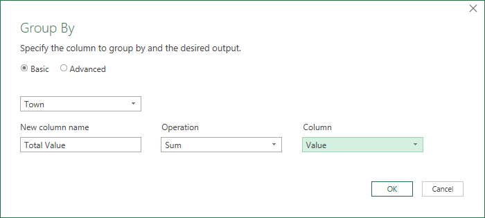
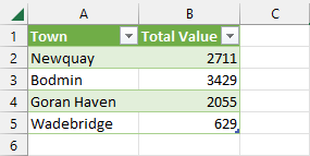
In the screenshot above, we have chosen to Sum the Value column into a column called Total Sales. After we click OK, it creates a summary report of sales by town (see the screenshot below).

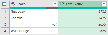
Now, we can click Home > Close & Load… to load the query as a Table on a new worksheet in Excel.

If we want every value to have a town, we must add Mega Mart and Wilson’s of Greenvale to the Customers table. After performing this and refreshing the data, we have a complete summary of sales by town.

Types of joins

In the example above, we used the Left Outer join. Before we look at another example, let’s take a few minutes to think about the other types of joins.

Joins enable us to compare lists, then return values accordingly. Thankfully, the descriptions provided for each join are a good summary of what it does.

Outer Joins

Outer joins return all the rows from one or both lists. We can select either Left, Right or Full, depending on which list should return all the rows.

• Left Outer: Returns all items from the first list and the matching items from the second list.
• Right Outer: Returns all items from the second list and the matching items from the first list.
• Full Outer: Returns all items from both lists.

Inner Join

An Inner join returns only items that exist on both lists. If the first or second list has items not on the other list, these are excluded from the result.

Anti Joins

Anti joins return the items which do not match any values on the other list.

• Left Anti: returns any items on the first list that have no matches on the second list
• Right Anti: returns any items on the second list that have no matches on the first list

This is all powerful stuff and proof that Power Query can achieve more than VLOOKUP, INDEX/MATCH, or even XLOOKUP.

Lookup value from another table with an approximate match

Now it’s time to consider calculating an approximate match. Before we start, if you’re unsure what this means, please read my post about Approximate Match here.

In this example, we calculate the value of a rebate due to a customer based on the sales value. Customers with sales greater than:

• £500 receive a 2% rebate
• £750 receive a 5% rebate
• £1,000 receive a 10% rebate

These thresholds are included in the Rebates query.

As we saw above, the value returned by the merge transformation is null unless there is an exact match. Therefore, a merge returns a value only if a customer has sales of precisely 500, 750, or 1000. So, we need to undertake a few more steps to make this function correctly.

To work along with this Example, add another version of the Sales table into Power Query.

With the new Sales query selected, click Transform > Group By.

When the Group By dialog box opens, make the following selections:

• Group by: Customer
• New column name: Total Sales
• Operation: Sum
• Column: Value

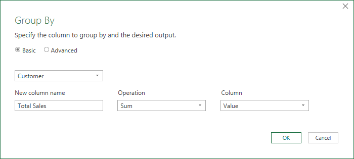
Click OK. The Preview Window now displays the following table, with the total sales by customer.

In the last example, we created the merge as a new query. This time, to demonstrate another method, we will add the Merge as another step to an existing query. Click Home > Merge Queries.

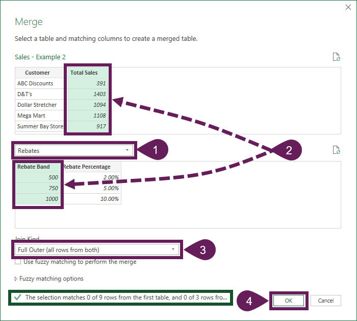
In the Merge dialog box

1. Select the query to merge with the selected query (Rebates in our example).
2. Select Total Sales from the Sales query and Rebate Band from the Rebates query.
3. Select Full Outer as the join kind.
   Note: At the bottom, it shows 0 matches in both tables. Don’t worry; this is OK for this scenario.
4. Click OK.

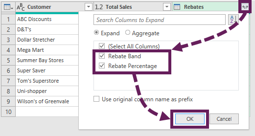
Expand the Rebates column, include both columns, then click OK.

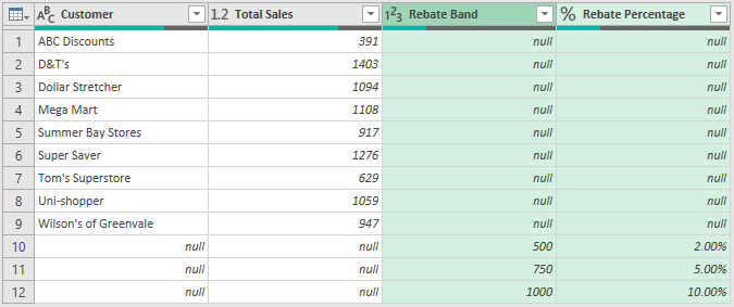
The Preview Window now looks like this:

Next, we need to combine the Total Sales and Rebate Band columns into a single column. For this, we will write an if statement. We could use the Conditional Column feature, but I find it easier to write it as a formula. Click Add Column > Custom Column.

In the Custom Column dialog box, provide a column name and enter the following text in the formula box:

if [Total Sales] = null then [Rebate Band] else [Total Sales]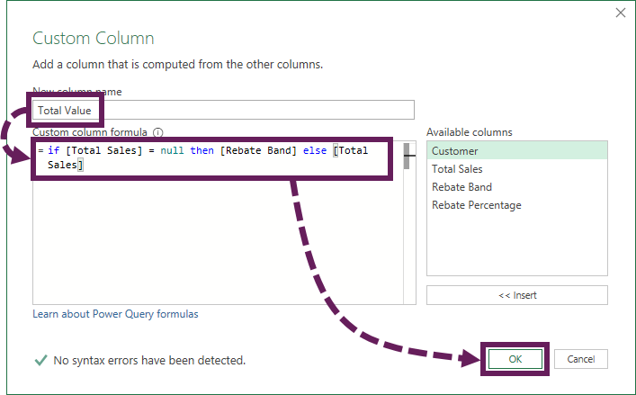

Power Query uses a different syntax to Excel for writing formulas, but hopefully, it’s understandable just by reading the text. We cover Power Query if statements in more detail in another post: Power Query if Statements.

Let’s make a few more transformations:

• Sort the new column by selecting the column header, then click Home > A-Z.
• Select the Percentage column and click Transform > Fill (dropdown) > Down.

The Preview Window should look like the following:

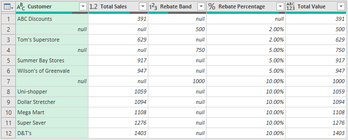
In the Rebates Percentage column, we need to replace null with 0. Click Transform > Replace Values and use the following:

• Value to find: null
• Value to replace: 0

You will notice that every customer now has a Total Value and a Rebate percentage. This means we can calculate the rebate value.

There are just a few steps remaining to tidy up the query:

• Filter out the null values from the Customer column
• Remove all columns except the Customer, Total Sales, and Rebate Percentage.

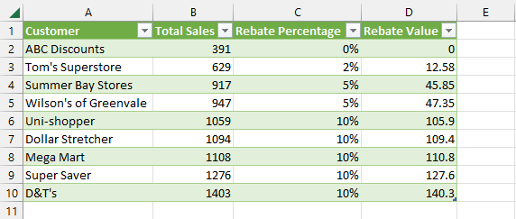
Finally, let’s finish by calculating the rebate value. Select the Total Sales and Rebate Percentage columns, click Add Column > Standard > Multiply.

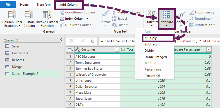
Rename the new Multiplication column to Rebate Value. Then we can Close & Load the table into Excel.

In this example, we have simulated an approximate match lookup using Power Query’s merge transformation.

Multiple matches

What happens if multiple items could match between tables? In this scenario, VLOOKUP, INDEX/MATCH, and XLOOKUP in Excel all return the first item found. Merge behaves differently.

Merge returns each instance of a matched item. So, for example, let’s assume we have two tables, one with Product information and another with Stock data about those products.

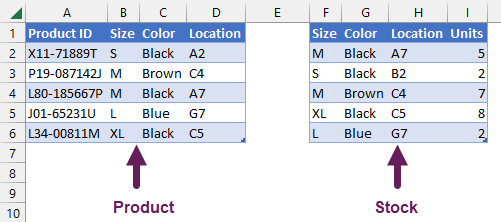
If we used a left outer merge on the Size column, the M-sized items would duplicate as there are two M’s in the lookup table.

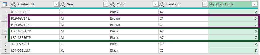
If you only want to match one item, remove the duplicate values from one of the tables before performing the merge.

Multiple Criteria Lookup

The great news is that Power Query does not restrict us to one list. Let’s say that we want to match three colums. That’s no problem.

The order in which we select columns determines which columns are matched. For example, look at the screenshot below. The columns selected in the first table were Color, Size, then Location (in that order). The numbers in the column header identify the order in which the items were selected. The columns selected in the second table must be in the same order.

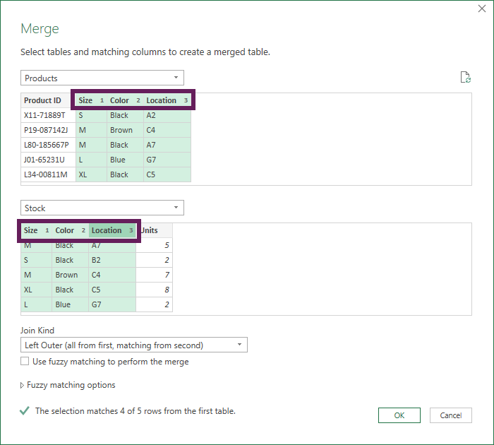
Using this approach, we can perform multi-column lookups between tables.

How easy is that!

Fuzzy Match Lookup

When looking at the Merge window in our examples, did you notice the option to Use fuzzy matching to perform the merge? This transformation uses an algorithm to match similar values. For example, with a Fuzzy Match, it is possible to match “Power Query” with “power-query”. You can’t do that with Excel’s lookup functions. We can even change the thresholds of how similar values must be before they match.

This is quite an advanced feature that requires careful consideration. Therefore, we won’t go into detail here, but you can find out more information in these posts:

• Excel University – Fuzzy match with Power Query
• Microsoft – Fuzzy match support for Get & Transform (Power Query)

Conclusion

Power Query does not have lookup functions, such as VLOOKUP, INDEX/MATCH, or XLOOKUP. However, using the merge transformation, we can still create exact and approximate matches to lookup values in another table.

Read more posts in this series

1. Introduction to Power Query
2. Get data into Power Query – 5 common data sources
3. DataRefresh Power Query in Excel: 4 ways  &  advanced options
4. Use the Power Query editor to update queries
5. Get to know Power Query Close & Load options
6. Power Query Parameters: 3 methods
7. Common Power Query transformations (50+ powerful transformations explained)
8. Power Query Append: Quickly combine many queries into 1
9. Get data from folder in Power Query: combine files quickly
10. List files in a folder & subfolders with Power Query
11. How to get data from the Current Workbook with Power Query
12. How to unpivot in Excel using Power Query (3 ways)
13. Power Query: Lookup value in another table with merge
14. How to change source data location in Power Query (7 ways)
15. Power Query formulas (how to use them and pitfalls to avoid)
16. Power Query If statement: nested ifs & multiple conditions
17. How to use Power Query Group By to summarize data
18. How to use Power Query Custom Functions
19. Power Query – Common Errors & How to Fix Them
20. Power Query – Tips and Tricks

---

What next?

Discover how you can automate your work with our Excel courses and tools.