In previous posts in this series, we’ve seen how to import external data from a single file, import all the files in a folder, and import data from a Table or range within the same workbook. But what if we want to import ALL the data within the same workbook? We are looking at that in this post: Use Power Query to get data from the current workbook.
Computers and humans think about data differently. People like to pre-categorize data into different areas. For example, we might keep January, February, and March data on separate sheets. However, computers are more efficient when data with the same structure is held in one table, with a separate column to identify each month. Power Query is amazing at getting data from the current workbook, which is in a human-understandable format, and transforming it into a computer-optimized format.
Table of Contents
Download the example file: Join the free Insiders Program and gain access to the example file used for this post.
File name: 0109 Get data from current workbook.xlsx
Watch the video

Get individual Tables or Ranges from the current workbook
Let’s start by looking at getting data from an individual Table or range into a query. The process depends on the location of the data:
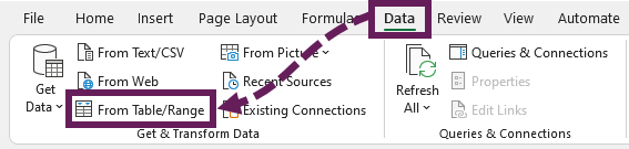
- Table – select any cell inside the table and click Data > From Table/Range
- Named Range – select the entire named range (if necessary, select it from the Name box), then click Data > From Table/Range
- Dynamic Array – select the top left cell in the array to display the spill range, then click Data > From Table/Range. In the background, Excel creates a named range and loads the data into Power Query
- Standard Range – select a cell inside a contiguous range and click Data > From Table/Range. Excel will convert the range to a Table before loading it into Power Query
Standard ranges are converted to Tables, and dynamic arrays have named ranges automatically created. Therefore, Power Query only has to work with two data objects, Tables and named ranges.
Next, we would make the necessary transformations. Then, when we are done, click Close and Load the push the data back into Excel.
However, before we move on, let’s look at the steps that Power Query creates when using these methods. For example, if we load a Table into Excel, the Source step might look like the following.
= Excel.CurrentWorkbook(){[Name="tblJanuary"]}[Content]What is happening here:
- Excel.CurrentWorkbook() – The Power Query function which gets data from the current workbook
- {[Name=”tblJanuary”]} – The result of the Excel.CurrentWorkbook function is filtered to only include items with tblJanuary in the name column
- [Content] – After the previous element there is only one row; this code element drills into the Content column of that row.
Now that we understand these elements, hopefully, you agree that Excel.CurrentWorkbook is the function we need for more advanced methods.
Microsoft’s guidance on the Excel.CurrentWorkbook function doesn’t contain a lot of information for us to work with.
Get data from the current workbook
Open the 0109 Get data from current workbook.xlsx file.
Based on our knowledge from the section above, we could load a Table or named range into Power Query, then edit the Source step to remove the parts of the M code we do not require.
= Excel.CurrentWorkbook(){[Name="tblJanuary"]}[Content]That is a nice simple method. Instead, we will expand our skills a bit and start from a blank query.
In Excel, click Data > Get Data > From Other Sources > Blank Query
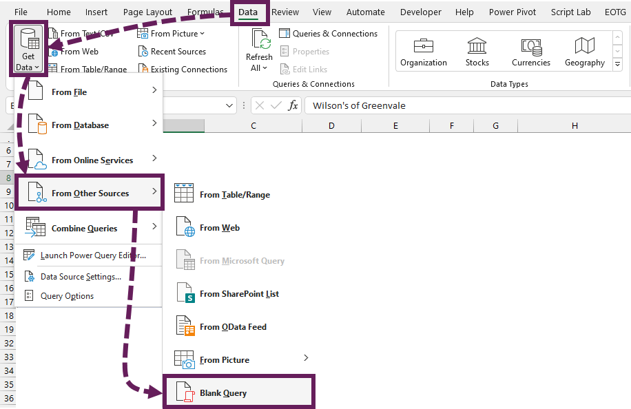
The Power Query Editor opens.
There is one step in the Applied Steps window, nothing in the Preview window, and most transformations are greyed out. While the Applied Steps window shows Source as the step, there is nothing in this step at present.
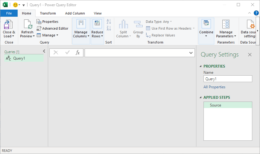
This truly is a blank query.
If the Formula Bar is not visible, click View > Formula Bar. Then, in the formula bar enter the following:
=Excel.CurrentWorkbook()Or, if you are feeling brave and want to use the Advanced Editor (Home > Advanced Editor), enter the following:
let
  Source = Excel.CurrentWorkbook()
in
  Source
Remember, M code is case-sensitive, so you’ll need to type the text exactly as shown above.
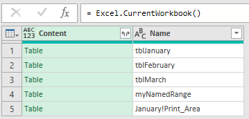
The Preview Window displays the data objects in the workbook:
- 3 tables (tblJanuary, tblFebruary, and tblMarch)
- A named range (myNamedRange)
- A dynamic named range (January!Print_Area)
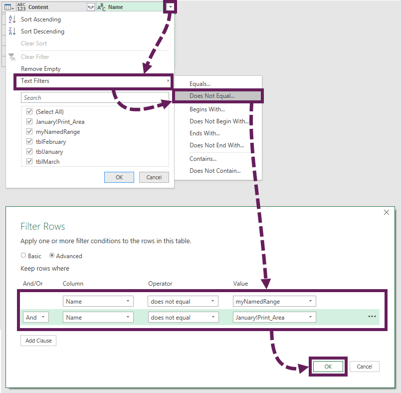
Let’s filter the name column to exclude the items we do not want.
Click Filter (icon) > Text Filters > Does not Equal…. In the Filter Rows dialog box, remove myNamedRange and Print_Area.
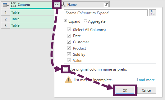
Next, click the Expand icon to drill into the workbook structure. Uncheck use original column name as prefix, then click OK.
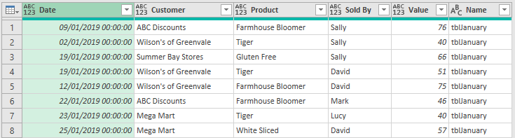
The Preview Window displays the combined data from all the selected data objects.
Complete the query with the following transformations:
- Remove the Name column
- Apply a data type for each column
- Give the query an appropriate name (I have chosen CombinedTable).
Click Close & Load to push the data into a new worksheet. You’ve just combined all the tables into a single view. Amazing, right?!
Warning: You don’t know it yet, but you’ve got a problem.
Filter out the query table
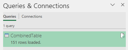
The Queries & Connections pane shows 151 rows loaded.
Don’t make any changes, but click Data > Refresh All again.
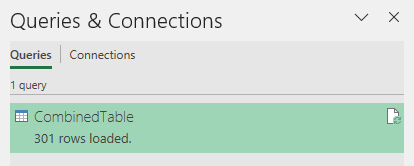
Err… what just happened. We’ve now got 301 rows, but we’ve not added any more data.
If we refresh the data again, we’ll have 451 rows. What is going on!!!!
Let’s head back into Power Query and see what’s going wrong.
Select the Source step in the Applied Steps box. Initially, there might not appear to be an issue. But once you click Home > Refresh Preview, the problem becomes clear. The preview window now shows this:
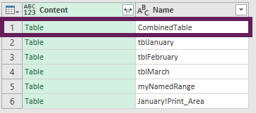
The CombinedTable query we created loads the data into Excel as a Table. Therefore, this Table is now included as a data object in the list. Each time the query is refreshed, it is combined with the other tables before being loaded back into Excel again. As a result, each time we refresh, the Table gets longer and longer and longer.
Let’s fix this problem.
We need to change our filter step. But what type of filter do we want? For example, do we want to remove the CombinedTable, or do we want to include tblJanuary, tblFebruary, and tblMarch tables only? This question determines what type of filter we should apply.
In this example, I have decided to include all items with the tbl prefix. Edit the previous filter step to include only items that begin with tbl in the Filtered Rows dialog box.
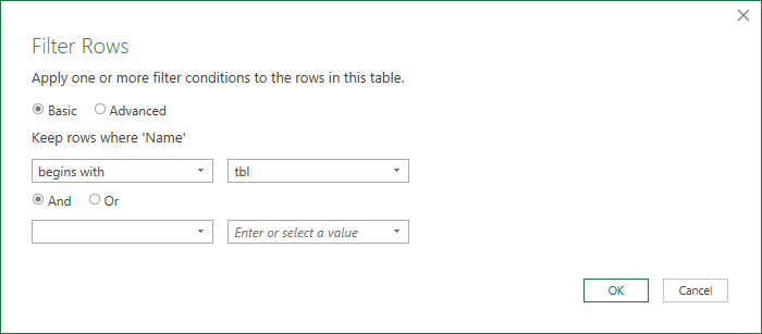
The M code in the formula bar will be:
= Table.SelectRows(Source, each Text.StartsWith([Name], "tbl"))This removes all the objects we don’t want, including the CombinedTable table. But, it allows other objects with a tbl prefix to be automatically included in the scope of the query.
Notes:
- Having standard naming conventions is critical to succeeding with this method.
- The ever-increasing data load is only an issue with Excel Tables; if the data is loaded to another source (e.g., Connection only), it will not appear as a data object using Excel.CurrentWorkbook.
Where is get data from sheets?
As we have seen, we can get data from Tables and named ranges, but what about sheets? That would be useful.
Unfortunately, at the time of writing, there is no option to get data from worksheets in current workbook. This is an omission in my opinion. It is a feature that has been requested from Microsoft many times. Maybe they will give it to us one day.
Conclusion
In this post, we have seen how easy it is to get data from the current workbook using Power Query. All it took was a little understanding of the Excel.CurrentWorkbook function.
When applying this method, if you load the data to an Excel Table, don’t forget to filter out the combined table to stop the ever-increasing data load.
Read more posts in this series
- Introduction to Power Query
- Get data into Power Query – 5 common data sources
- DataRefresh Power Query in Excel: 4 ways & advanced options
- Use the Power Query editor to update queries
- Get to know Power Query Close & Load options
- Power Query Parameters: 3 methods
- Common Power Query transformations (50+ powerful transformations explained)
- Power Query Append: Quickly combine many queries into 1
- Get data from folder in Power Query: combine files quickly
- List files in a folder & subfolders with Power Query
- How to get data from the Current Workbook with Power Query
- How to unpivot in Excel using Power Query (3 ways)
- Power Query: Lookup value in another table with merge
- How to change source data location in Power Query (7 ways)
- Power Query formulas (how to use them and pitfalls to avoid)
- Power Query If statement: nested ifs & multiple conditions
- How to use Power Query Group By to summarize data
- How to use Power Query Custom Functions
- Power Query – Common Errors & How to Fix Them
- Power Query – Tips and Tricks
Discover how you can automate your work with our Excel courses and tools.
The Excel Academy

Make working late a thing of the past.
The Excel Academy is Excel training for professionals who want to save time.