Filter All in Power Query

Filtering in Power Query reduces the table to include only those items which meet specific criteria. However, Power Query doesn’t have an option to filter to include all items. In Excel, we can use the asterisk ( * ) as a wildcard character to match any text. Therefore, if we want to include all items in a Filter, we just use a single asterisk. However, Power Query doesn’t have equivalent functionality. So, in this post, we will look at a method to create something similar to filter all in Power Query.

This post is in response to a question from an academy member who was asking about filtering a table.

“I need an ‘all’ option…so if they don’t select a name, then they get all the records.”

OK, let’s see how we can solve this.

Table of Contents

• The scenario
• Adding the filters to Power Query
• Applying the filter in Power Query
• Testing the solution
• Conclusion

Watch the video

Watch the video on YouTube.

The scenario

To demonstrate the approach, I have created a workbook containing two filters.

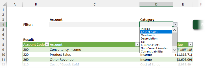
• Account allows us to select an account code
• Category allows us to select a category

The workbook includes a query linked to an external CSV file and loaded into a Table. The CSV file is included in the download file. To work along with the example, you will need to re-point the query to the source CSV file on your PC.

In the example workbook, these filters don’t currently do anything. But we want to create the functionality to filter by Account or Category, but if either is left blank, it will return all the items for that item.

Adding the filters to Power Query

The first step is to create two named ranges:

• Cell C4 = AccountFilter
• Cell D4 = CategoryFilter

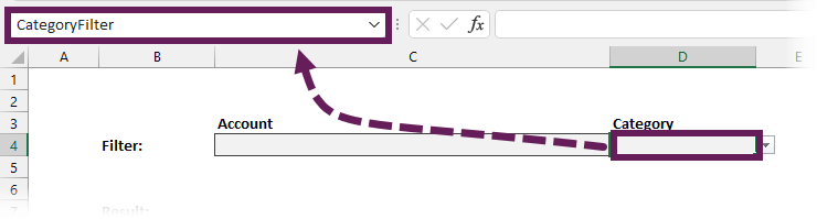
Now let’s add both of these named ranges into Power Query as parameters

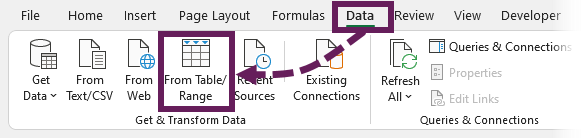
• Select cell D4 and click Data > From Table/Range from the ribbon
  
• Change the data type to text
• Replace the null values with a blank text string by clicking Transform > Replace Values
  
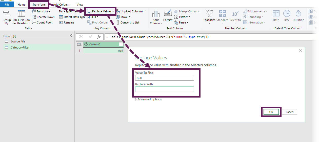
• Right-click on the blank cell and select Drill Down to get to a single value.
  
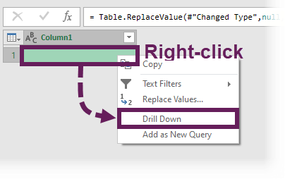
  Note: If the cell filter was blank, you will not see any values on your screen (that’s fine, don’t worry)
• Close and load this query into Excel as a Connection only.

Repeat these steps for the AccountFilter in cell D4.

Applying the filter in Power Query

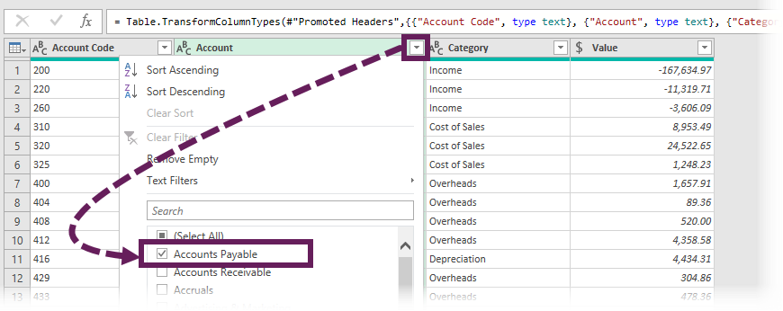
Go back into Power Query, in the source query, select the Account column and apply a text filter; use any text, it doesn’t matter.

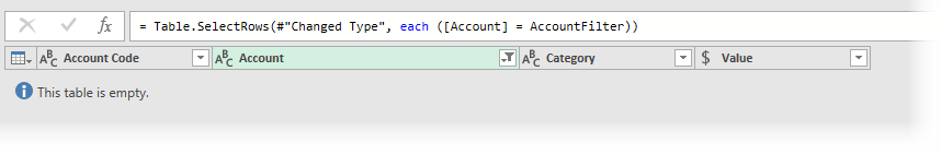
Next, in the Formula Bar, change the filter text string to be the AccountFilter query. To do this, change the following:

= Table.SelectRows(#"Changed Type", each ([Account] = "Accounts Payable"))

To this:

= Table.SelectRows(#"Changed Type", each ([Account] = AccountFilter))

If the filter was empty, the screen will now look like the following:

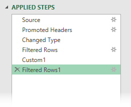
If you are working along with the example, the applied steps contain the following items:

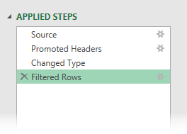
We can now add logic to the applied steps to return the filtered or unfiltered tables.

Click the Fx symbol to create a new step. Enter the following statement into the formula bar.

= if AccountFilter = "" then #"Changed Type" else #"Filtered Rows"

This is simply saying that if the AccountFilter is a blank text string, then return the table after Changed Type, (which is unfiltered), otherwise return the table after Filtered Rows (which is filtered). This creates the effect of a blank filter returning all the items.

Repeat the actions above for the Category column and the CategoryFilter query.

Before creating the second if statement, the applied steps will be:

Therefore, the if statement will be:

= if CategoryFilter = "" then Custom1 else #"Filtered Rows1"

Finally, close and load the Source query as an Excel table.

Testing the solution

Now, all we need to do is test it out. First, enter some values into either filter box, then click Data > Refresh All from the ribbon.

If either or both cells are blank, no filter is applied to the final table for those filters.

The screenshot below shows a filter on the Category, but no filter applied to the Account column.

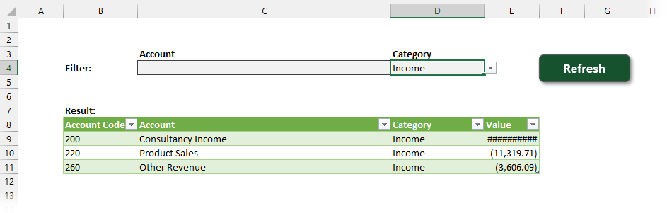
I have added a refresh macro button and data validation drop-down lists in the example file. However, the data validation list illustrates how the solution might work; it is not dynamic, so it will not pick up any extra values.

Conclusion

Power Query doesn’t have filtering by wildcards for us to include all items. But with a little bit of logic, we can create a similar effect.

And maybe in the process, you’ve learned that you can type directly into the formula bar and easily return the query’s status after each applied step.

---

What next?

Discover how you can automate your work with our Excel courses and tools.