Power Query – Tips and Tricks

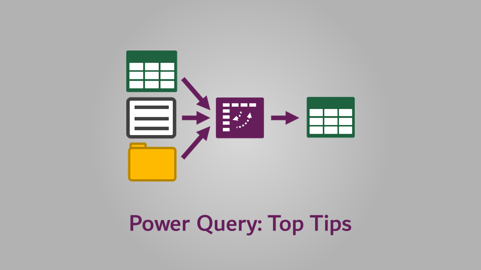
It’s now time to bring this Power Query series to a close.  And where better place to end than with some tips and tricks to help you to succeed.

Change the default Close & Load options

Power Query’s default Close & Load options assume we want to load the data into an Excel table.  As you progress with Power Query, this will become less and less the norm.  Actually, as you progress along your “Power” journey, you’re more likely to use data within Power Pivot, which requires loading into the data model.

To change the default Close & Load options, open the Power Query editor, then click File -> Options and settings -> Query Options.

In the Query Options window, select the Global: Data Load option.

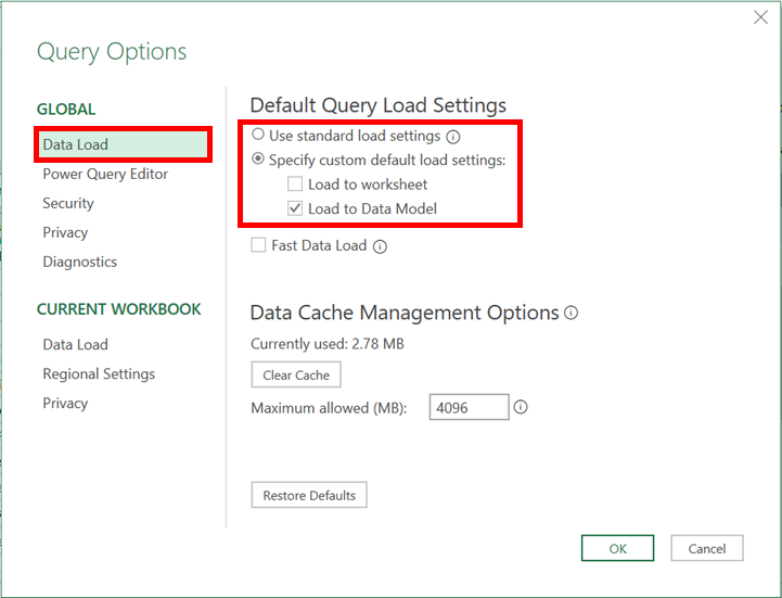
In this dialog box we find the specify custom default load settings option:

• Load to worksheet – if checked the data loads to the worksheet, if unchecked, it loads as a connection only.
• Load to Data Model – if checked the data loads into the data model, if unchecked, nothing loads into the data model.  To use the data in Power Pivot, this option must be checked.

Selecting use standard load settings is equivalent to checking load to worksheet, and unchecking the load to Data Model.

Give steps a meaningful name

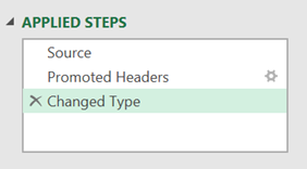
I am guilty of not following my own advice here.  Renaming steps to have a meaningful description is such a time saver.  It may not seem it at the time, but in the long-run, it will be.  It is so easy to have queries where the applied steps look like this:

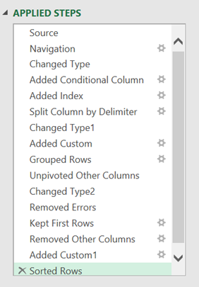
What did each of those steps do?  There are way too many to remember, so we’ll have to keep looking back at the Preview Window and Formula Bar in an attempt to work out what we did.  If only we had renamed the steps when creating the query.

Renaming the steps is easy — Right-click on the step name and select Rename from the menu.

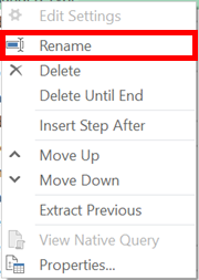
This also changes the name of the step in the Advanced Editor.

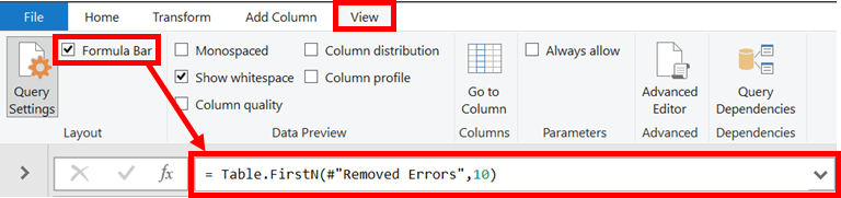
Always have the Formula Bar visible

The Formula Bar is the perfect balance between the complexity of the Advanced Editor window and the simplicity of the main user interface.

Seeing the M code helps us to:

• Learn and appreciate what Power Query is doing in the background
• Quickly make small code edits where needed

If you’re coming from an Excel world, the Formula Bar is a familiar element of the window.  We might not understand everything within it, but that doesn’t mean it’s not useful.

To enable the Formula Bar click View -> Formula Bar from within the Power Query editor.

Prevent auto-detect data type

Every time we import data, Power Query guesses the type of data each column contains.  Based on this guess, a new step is added to the applied steps list.

Also, if the data is unstructured, such as a CSV file, or a named range, the first row will be promoted to the header row automatically.

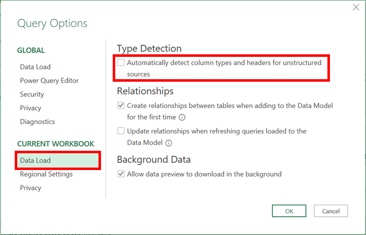
We can find ourselves regularly deleting these steps.  Therefore, it may be faster and easier to disable auto data type detection  Within the Power Query editor, click File -> Options and settings -> Query Options.

In the Query Options window, select the Current Workbook: Data Load group.

Remove the tick from Automatically detect column types and headers for unstructured sources, then click OK.

Any queries created will now include only the Source step.  It’s up to us to decide if and when to promote headers and data types to use.

Use Go To Column

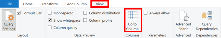
While working with a table containing lots of columns, it can be time-consuming to find the column we want; moving back and forth with the horizontal scroll bar is not fast.  Using the left and right cursor keys can be a useful, but there is a better way, called Go to Column.

The Go to Column icon is hiding away on the View ribbon (which is the one we rarely use).  Click View -> Go to  Column.

The Go to Column dialog box is simple and easy to use.

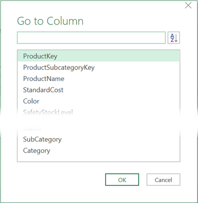
There is no multi-select or complex selections, simply select the column name, then click OK (or double-click the column name to avoid clicking OK).

The box at the top allows us to search for any text string. Next to that is the icon to sort in alphabetical or natural order.  Searching does not have any effect on the source data; it’s purely for finding a column.

Create folders for grouping queries

The more queries we have, the more cluttered the Queries & Connections pane and query list become.  The examples we have used in this series have been relatively straight forward with just a few queries.  But in the real world, there are likely to be a lot more.

It is an excellent idea to organize queries by putting them into groups.  This is what Power Query does when it combines multiple files.

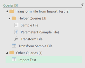
How you decide to organize the groups is up to you.  But Parameters and Custom Functions are ideal candidates to put into their own folder.  Also, as you advance in Power Query, you may start to create separate queries for extracting, transforming, and loading data; these are also useful organizational groups.

Folders can be created in the Queries and Connection pane, or the Query list.

Query list (in Power Query Editor)

If using the Queries list in the Power Query Editor, Right-click on the list and select New Group.  Give the group a name, then click OK.  A new folder will be created.

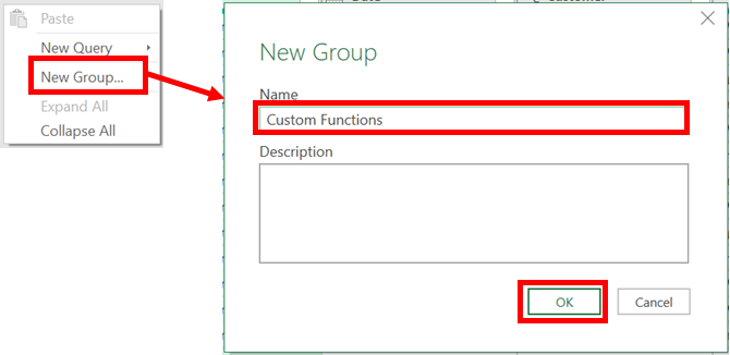
Drag the queries into the folders as required.

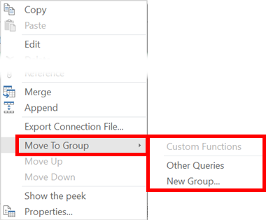
Queries & Connection (in Excel)

The process for creating folders in the Queries & Connections pane is slightly different. Right-click on the list and select Move To Group to reveal the options for creating folders or movings queries.

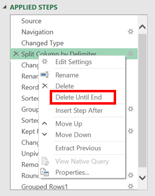
Delete steps until end

Building effective queries takes practice.  Even then, we can find ourselves following a particular path, only to find out that the choice we made 15 steps ago wasn’t the best decision. Therefore, all the subsequent steps are built on a sub-optimal choice.

We could delete each step one-by-one to get back to the point before the decision; this will take a lot of clicks.  Instead, we can achieve it with just two clicks :-).

In the applied steps list, right-click on the first step we wish to delete and select Delete Until End.  All the subsequent steps will be removed.

Split a query into two

Sometimes the first part of a query is ideal as the first steps for another query.  You might be tempted to build another query which contains the same steps… but that is a bad idea.  Instead, it’s better to split the query into two parts, then use the first part as the source for both.

Right-click on the step where you want to split the query, then click Extract Previous (a slightly strange name in my opinion).

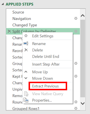
Give the query a new name, and click OK.  You’ll now have two queries:

1. The first part of the initial query
2. The second part of the initial query, which uses (1) as its source

The first part of the initial query can now be used as the source for others.

Copy and paste queries to a new workbook

If you’ve created a useful query, why only use it once?  It can be easily copied and pasted between workbooks.

In Excel’s Queries & Connections pane, right-click on the query, and click Copy.  In the target workbook, right-click in the Queries & Connections pane and click Paste.  It’s that easy.

This will paste the query itself, along with any other referenced objects.  Obviously, if there are data sources used from within the source workbook, these will need to be repointed, to data in the target workbook.

Using comments

Much like renaming steps, comments are one of those things we think we will get around to at a future point… but we never do.  Within a few days, we have forgotten why we made certain decisions or what specific pieces of code are intended to do.  When this happens, we waste a lot of time trying to understand our previous decision-making process.  This is why comments are so important.

Inserting comments into the Advanced Editor / Formula Bar

A single-line comment in the Advanced Editor is denoted by two slashes ( // )

// This is a single line comment

Multi-line comments involve a mix of slashes and asterisks as shown below:

/* This is a multi-line comment: line 1
line 2
line 3 */

Comments entered using these methods are only visible in the Advanced Editor; they are not shown in the Formula Bar.  Comments can be added into the Formula Bar, but once another step is selected, these comments are no longer visible.

Inserting comments into the step properties

If we right-click on any step, there is the Properties… option in the menu.  Click that to enter the Step Properties dialog box, then enter the comment in the description box.  Finally, click OK.

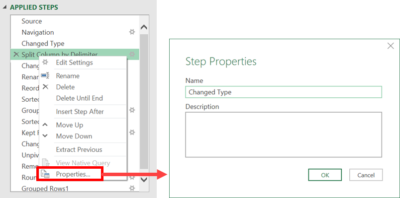
Any text entered into the Description box is included within the Advanced Editor as a single line comment.

Thank You

That’s it for this Power Query series.  If you’ve been following along, I hope you now feel capable enough to play around with Power Query.  After you’ve been using Power Query for a bit, I recommend that you come back and work your way through again.  It’s incredible the number of things which will make more sense the second time around.

Thank you for reading and following along 🙂

Read more posts in this series

1. Introduction to Power Query
2. Get data into Power Query – 5 common data sources
3. DataRefresh Power Query in Excel: 4 ways  &  advanced options
4. Use the Power Query editor to update queries
5. Get to know Power Query Close & Load options
6. Power Query Parameters: 3 methods
7. Common Power Query transformations (50+ powerful transformations explained)
8. Power Query Append: Quickly combine many queries into 1
9. Get data from folder in Power Query: combine files quickly
10. List files in a folder & subfolders with Power Query
11. How to get data from the Current Workbook with Power Query
12. How to unpivot in Excel using Power Query (3 ways)
13. Power Query: Lookup value in another table with merge
14. How to change source data location in Power Query (7 ways)
15. Power Query formulas (how to use them and pitfalls to avoid)
16. Power Query If statement: nested ifs & multiple conditions
17. How to use Power Query Group By to summarize data
18. How to use Power Query Custom Functions
19. Power Query – Common Errors & How to Fix Them
20. Power Query – Tips and Tricks

---

What next?

Discover how you can automate your work with our Excel courses and tools.