
If you’re like me, you build Power Query solutions in a test environment first; then, when ready, it’s released into the wild. This means the paths of all source files must be updated. Or maybe you’re a consultant who creates solutions for others; when you distribute the workbook to your client, you have to provide them with complicated instructions on how to update the data sources for their environment. Wouldn’t it be better if the source could be linked to a cell value that we, or a client, could easily update? Yes, it would! So, in this post, we’re going to look at how to do that; how to change the Power Query source based on a cell value.
I have written about changing Power Query sources before (Power Query: Change the Source Data Location). In that post, I show the manual method and a method using parameters. What I’m about to show you is an even easier method.
I must say “Thank You” to Celia Alves for sharing this technique on a recent online meetup.
Table of Contents
Download the example file: Join the free Insiders Program and gain access to the example file used for this post.
File name: 0021 Power Query – Change source based on cell value.zip
The download file includes three files:
- Source file – the data loaded into Power Query
- Start file for the example
- Completed file for the example
Watch the video:

The scenario
I’m not going to provide details on how to load the source data into Power Query; I’m assuming you already know how to do that.
If you’re using the example files, the data loaded from the source file looks like this:
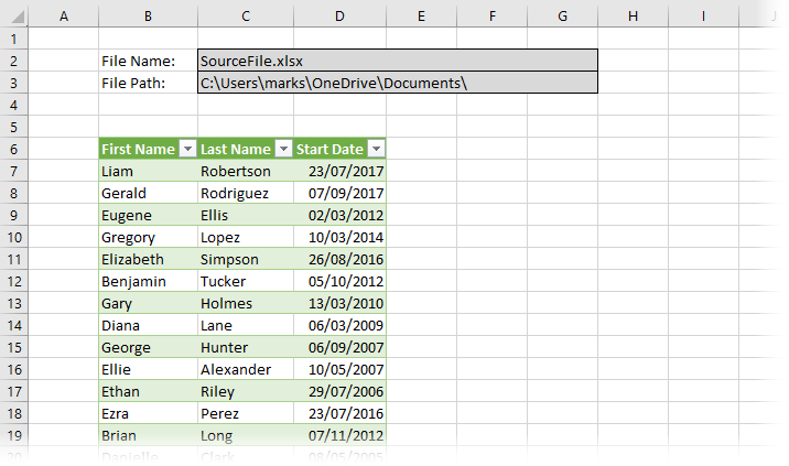
Cell C2 contains the file name, and cell C3 contains the folder path. These are not currently linked into anything; it is presently just text in a cell. But by the end of this post, these cells will be connected to Power Query.
These are file locations on my PC, so will not work for you. Change the file name and folder path to the location of your source file.
NOTE: A common error is to forget the backslash at the end of the folder path.
Create named ranges
Now, create two named ranges:
Select cell C2 (the file name) and create a named range called FileName. To do this type the name of the named range into the name box and press Enter.
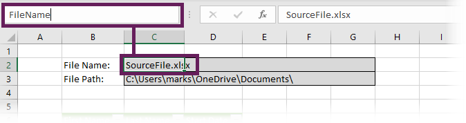
Next, we repeat the step above for the file path. Select cell C3 (the file path) and create a named range called FilePath.
We will be combining these two named ranges in Power Query’s M code. So, make sure they form a valid file path.
Use named range within M Code
Now we just need to use the named ranges in our query.
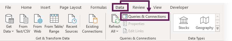
Open the Queries and Connections pane by clicking Data -> Queries & Connections.
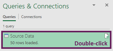
Double click the name of the query to open the Query Editor.
 ]
]
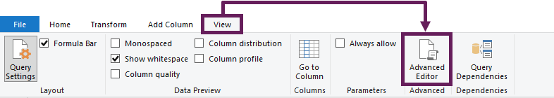
In the Power Query editor, click View -> Advanced Editor.
Reference named ranges in M code
We will add new steps directly after the let statement.
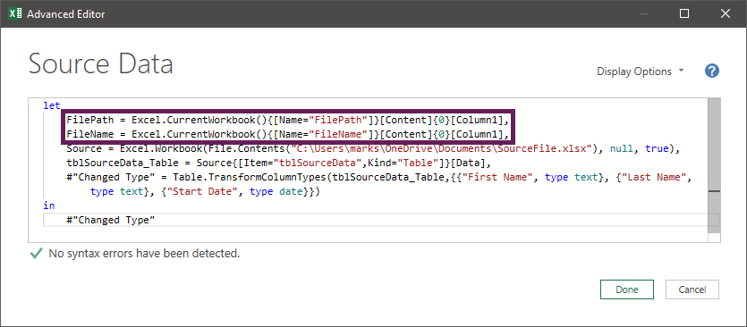
FilePath = Excel.CurrentWorkbook(){[Name="FilePath"]}[Content]{0}[Column1],
FileName = Excel.CurrentWorkbook(){[Name="FileName"]}[Content]{0}[Column1],
These lines of M code are effectively the same, but one is for the file path and one for the file name. The code breakdown for the first line is as follows:
- FilePath = : The name of the step in Power Query
- Excel.CurrentWorkbook() : Power Query function which uses data from the current workbook
- {[Name=”FilePath”]} : The name of the named range
- [Content]{0}[Column1] : Uses the first row and the first column from the table of the named range
REMEMBER: Make sure each line of code in the Advanced Editor is finished with a comma.
In this example, we have two named ranges, but we can create as many as we need.
Use named ranges as source
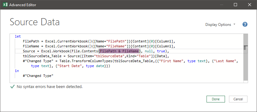
Finally, we need to insert the FilePath and FileName steps into the Source step.
Replace this:
Source = Excel.Workbook(File.Contents("C:\Users\marks\OneDrive\Documents\SourceFile.xlsx"), null, true),
with this:
Source = Excel.Workbook(File.Contents(FilePath & FileName), null, true),
Click Done to close the Query Editor. Then Close and Load the data back into Excel.
Assuming we’ve done everything correctly, the data in the query is now linked to the cells. We can change the values in cells C2 and C3, then click refresh and Ta-dah! The data will refresh to the new source file. We’ve managed to change the Power Query source based on a cell value.
Make the file path dynamic (not for OneDrive)
If the source files are contained in the same folder as the workbook containing the query, it is possible to use a dynamic file path. Try entering the following into cell C3.
=LEFT(CELL("filename",$A$1),FIND("[",CELL("filename",$A$1),1)-1)
The formula will automatically update to show the correct file path.
Notes:
- The workbook containing the query must be saved
- Workbooks saved to OneDrive will display the https URL, rather than the local file path, making this method difficult to use without further development
Conclusion
That’s it, we’ve learned how to change the Power Query source based on a cell value. All it takes is a few named ranges, and a few short lines of M code.
Now any user can easily change the cell to re-point the query to the correct source data location. They don’t even need to open Power Query, or understand how it works.
Discover how you can automate your work with our Excel courses and tools.
The Excel Academy

Make working late a thing of the past.
The Excel Academy is Excel training for professionals who want to save time.
Great page!
Thanks Ed 🙂
Thank you !
I could make it work for a file on SharePoint, by replacing “File.Contents” with “Web.Contents” in the Source, as below
Source = Excel.Workbook(Web.Contents(FilePath & FileName), null, true),
Thanks JM – Great add.
Thank’s for the article, very usefull.
OMG I have been looking for this for ages… THANK YOU
Thank you for the article; very useful. I have seen where a “Refresh all” can update the query automatically with a macro running on change of a cell value, but looking to only do this once data input is completed in more than one cell to then the macro to update – and not update on when each cell changes.
Is this possible?
It’s possible. But would need to be coded specifically to your circumstances. It will depend on exactly which cells and in what order and how you decide what a change is.
If you don’t know how to do it, I would recommend a service like Excel Rescue (https://excelrescue.net/works-with/exceloffthegrid)
how do i specify the Sheet?
Hi Patrick – The sheet is defined in the Named Range (i.e., it refers to a specific range on a specific sheet).
Can you elaborate on this/show an example?
super introduction to power query! this has helped me a lot
2 supplementary questions:
– in the video at 3’50” the advanced editor appears with text highlighting and hints, similar to notepad++. any tips on how you implement this within power query? (I defined within my NP++ the language M as UDL).
– in MS Query you can define when the cell value for the query parameter changes that the query is refreshed. any tips how to realize this with PowerQuery (VBA in Excel Workbook)?
thanks a lot
Hi Martin,
The formatting of the editor is dependent on which version of Excel you’ve got. I can’t recall which build version this feature was released on.
In terms of automatically refreshing a PowerQuery, you will need to use the worksheet change event in VBA to trigger the refresh. I don’t have any content which specifically addresses this, the closest content I have is this video: https://www.youtube.com/watch?v=rDkWIDU7_Fo
Hi,
Thank you for the tip. Made changes to get all files from a folder, working for me.
FILEPATH = Excel.CurrentWorkbook(){[Name=”FILEPATH”]}[Content]{0}[Column1],
Source = Folder.Files(FILEPATH),
Hi – can you describe how one might update this to run as a programmed macro tied to a button click? The vba seems to be having challenges with the curly bracket? Thanks very much.
Hi Andy – I’m not sure why you need to use curley brackets in the VBA code. Once the link is set-up it should be a simple refresh process.
Check out this post, it shows how to auto-refresh the Power Query source when a cell value changes.
https://exceloffthegrid.com/auto-refresh-power-query/
Thank you – great post! Appreciate your very thoroughly step-by-step, works great and helped me a lot.
Dear Mark,
Thanks the brilliant and clear article. It helps a lot.
Preciously I had tried the following idea:
1) create a query (FileLocation) to drill down a table in the excel file as
C:\PQ\sample.xlsx
2) modify M code to
Source = Excel.Workbook(File.Contents(FileLocation), null, true)
But as you might have known, this trick did not work. Do you know what went wrong? And is it possible to fix it directly in M code?
Thanks again for sharing your valuable knowledge.
Thank you! And how about a source file is a folder or a txt/csv file?
The principles are exactly the same, no matter what the source is.
Same principles and methods apply
Excellent!! Thank you
You mentioned as many ranges can be used as needed. I tried pulling in multiple files from the same file path using a different file name and named range, but am having trouble. How would i apply this to bring in multiple files?
I found my error. Thank You!
Good news 😊
Brillaint. Been searching for so long to find this. Coupled this with another query which invokes the user name to replace the user in the path (we use Dropbox). So the FieldPath is automatically updated with the right user name upon ‘Refresh All’ so any user (provided they use the same drive letter for their Dropbox) can refresh. Found this which can be pasted directly into a new query. Might be useful:
() =>
let
Source = Folder.Contents(“C:\Users\”),
#”Expanded Attributes” = Table.ExpandRecordColumn(Source, “Attributes”, {“Hidden”, “Directory”, “ChangeTime”}, {“Hidden”, “Directory”, “ChangeTime”}),
#”Filtered Directories not hidden” = Table.SelectRows(#”Expanded Attributes”, each ([Directory] = true) and ([Hidden] = false)),
#”Removed Errors” = Table.RemoveRowsWithErrors(#”Filtered Directories not hidden”, {“ChangeTime”}),
#”Filtered Rows” = Table.SelectRows(#”Removed Errors”, each ([Name] “Public”)),
#”Username” = #”Filtered Rows”{0}[Name]
in
#”Username”
Thanks Rupert, that is really useful stuff. 🙂
Excellent resource! Exactly what I needed. Thanks! (Modified the edit slightly to get it to grab a different sheet from the same source file based on a cell value, but the logic is the same).
Yay!! Great News. I’m glad it helped 😀
Thanks for this post. This did the trick for me with some modifications. I am sourcing a file on Dropbox, and the filepath is dynamic based on the user.
1. Remove the space between FilePath & File Name in below line:
Source = Excel.Workbook(File.Contents(FilePath & FileName), null, true),
2. Populated FilePath with expression to make dynamic:
=@fn_directory&”\”
This
Dropbox as a source, I’ve not tried it. That’s useful to know 😀
I am using Excel for Mac and when I get to the step where I press “Close and Load,” I receive the following message: “An on-premises data gateway is required to connect.”
Any ideas on how I can overcome this?
Sorry, I’ve never used it on a Mac. You might want to try the Microsoft Answers community.
This is a life saver. Thank you Mark! <3
You’re welcome 😁
I am getting an error
DataFormat.Error: The supplied file path must be a valid absolute path.
Can you help? I have a url string for example
I:\Folder1\Folder2\Folder3\ExcelFile.xlsx
In this example, Folder2 changes via formula
All the references and url is correct, I just keep getting that error.
I’ve made the FileName and FilePath dynamic so I don’t have to copy and paste each time I add the connection to a new file!
FileName
=TEXTAFTER(SUBSTITUTE(TEXTBEFORE(CELL(“filename”,A1),”]”),”[“,””),”\”,-1)
FilePath
=TEXTBEFORE(SUBSTITUTE(TEXTBEFORE(CELL(“filename”,A1),”]”),”[“,””),”\”,-1)&”\”
There’s probably a better way to capture the final slash in the path, but this works for now.
RE: I’m creating a PQTOC that I can use in any file
Good work. the CELL function is very popular for that.
Is there any way to dynamically change exchange.contents source from within Excel too?
Many thanks
You would need to add an if statement in the Power Query M code to switch between the different options.