How to get data into Power Query – 5 common data sources

OK, let’s get started with Power Query. The first thing we need to do is get data into Power Query. In this series, it is our first real look at Power Query; we are also going to use this as an opportunity to explore the user interface.

This post is structured into two main parts:

1. Using data in the same workbook – this includes an Excel Table, named range, dynamic array, or worksheet range
2. Using data from external files and external workbooks – this includes CSV files, text files, or Excel workbooks

As we work through the examples, I hope you will see that getting data into Power Query is easy.

There are many other connectors for loading data into Power Query, the key connectors we will cover in later sections. The principles for loading data will be relevant for any connectors we do not include.

Please note that Microsoft is constantly updating Excel and Power Query. Therefore, depending on your specific build version of Excel, various actions’ names, locations, and options may differ slightly from the examples shown in this post.

Table of Contents

• Using data in the same workbook
• Importing data from Tables
• Importing data from named ranges
• Importing data from dynamic arrays
• Is it better to use named ranges or Tables?
• Importing data from external files and Excel workbooks
• CSV File
• Text File
• Excel workbook sheets
• Wrap-up

The download includes 5 files:

• Example 1 – Table.xlsx
• Example 2 – Named Range.xlsx
• Example 3 – CSV.csv
• Example 4 – Text.txt
• Example 5 – Excel Workbook.xlsx

Using data in the same workbook

The easiest place to start is getting data from the same workbook. Power Query recognizes two sources from the same workbook, Excel Tables, and named ranges. We can also obtain data from dynamic array spill and standard ranges using these two sources.

Importing data from Tables

Let’s start by looking at Excel Tables; they are the easiest to work with as Power Query views it as a structured format.

It is important to note that I am using “Tables” to refer specifically to the Excel Table feature and not data contained within normal cells. Tables are a vital element of how Excel likes to store data, and they work incredibly well with Power Query.

The following uses Example 1 – Table.xlsx from the downloads.

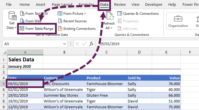
To get an Excel Table into Power Query:

• Select any cell in the Table
• Click Data > From Table/Range

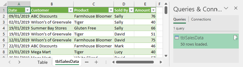
The Power Query window will open. As this is our first look at the user interface, we will spend some time understanding what’s here.

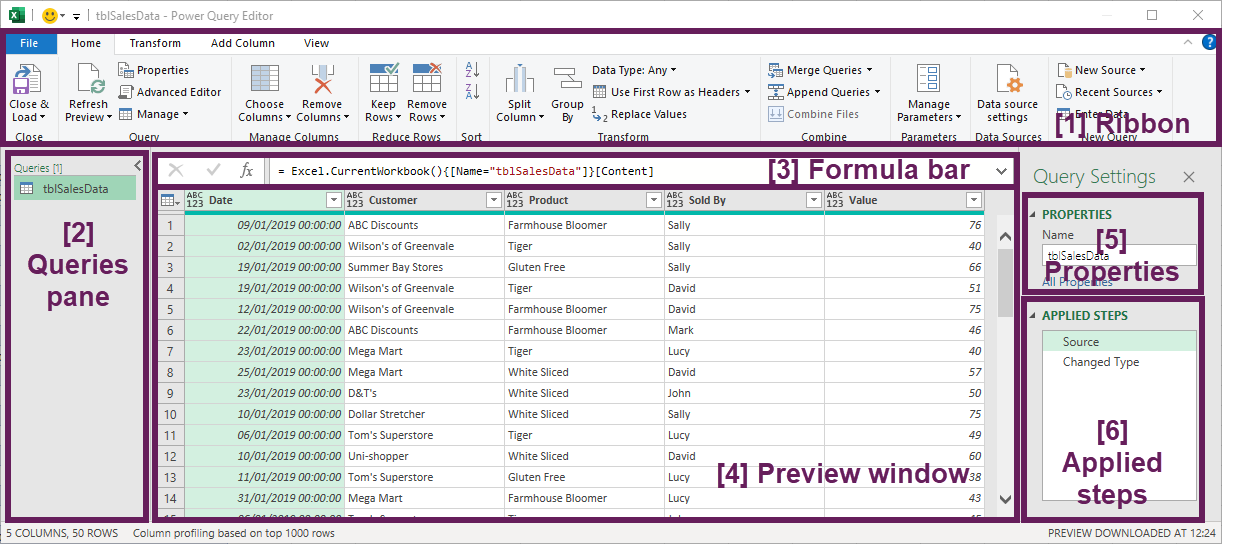
1. Ribbon – Similar to Excel, the ribbon contains the main commands grouped into separate tabs. We will be using the ribbon throughout this series. Even though it might look a bit strange now, you will get to see the most common commands in action.
2. Queries pane – This lists all the queries within the workbook. The small arrow at the top can be clicked to expand or hide the pane. Depending on your version of Excel, this may be hidden or expanded by default.
3. Formula Bar – The formula bar shows the code for each transformation step. Depending on your version of Excel, this may be hidden by default. Click View > Formula bar to make it visible.
4. Preview – This area shows a preview of our data based on the selected step within the applied steps box. We can access many of the column-specific transformations by right-clicking on the column headers within this section.
5. Properties – This is where we name the query. There is nothing helpful about the name Query 1, so giving your query a meaningful name is important. You want to use a name that describes what it does without looking at the steps.
6. Applied steps – Each transformation action you take is listed in the Applied Steps. In this box, it is possible to add, remove, edit and rename steps.

Understanding the applied steps

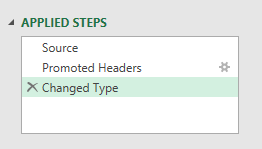
The applied steps window already contains a small list of items. These steps are Excel’s attempt to automatically transform the data based on what it believes we want to do.

Source – Identifies the source data (e.g., the Table on the worksheet)

Changed Type – Excel has analyzed the data and tried to apply the correct data type to each column.

These steps have been applied automatically by Excel. Be warned, the automatic steps are not always correct. I have found the Change Type step can often cause frustrating errors later, which are incredibly difficult to find. Sometimes it is easier to delete the change type step and change the data types column-by-column.

When we undertake any transformation actions, these are all added to the applied steps list.

Clicking on each step within the applied steps box changes the preview window; it lets us see how each step changes the data.

M Code

M is the language Power Query uses to record each transformation that occurs. It is a function-driven language, so it has some similarities to Excel. However, given that the purpose of Power Query is to transform data rather than calculate values, the functions are very different to Excel.

Let’s take a brief look at the M code, to see how Power Query has recorded the steps. Don’t worry, we will not be spending much time looking at M code, but it will help us understand how Power Query works and how to make more advanced edits to queries when we have more experience.

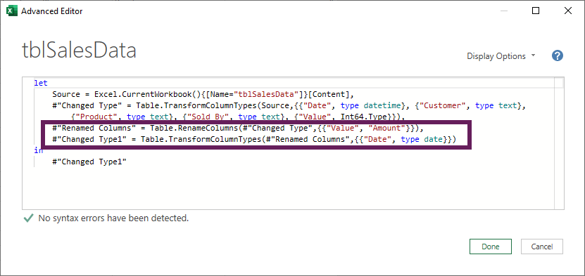
Click Home > Advanced Editor (an alternative method is View > Advanced Editor).

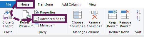
The Advanced Editor window appears, showing the code for the applied steps.

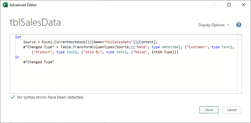
We will briefly examine the code and compare it to the applied steps. We won’t spend much time looking at M code, but it’s worth taking a brief look to understand what Power Query is doing.

let

let is a keyword to identify the beginning of a code segment

Source = Excel.CurrentWorkbook(){[Name="tblSalesData"]}[Content]

Source is determining which Excel Table to use as the source data. If we want to change the Query to look at a different Table, we could change the text “tblSalesData” to the name of the new Excel Table.

#"Changed Type" = Table.TransformColumnTypes(Source,{{"Date", type datetime}, {"Customer", type text}, 
{"Product", type text}, {"Sold By", type text}, {"Value", Int64.Type}})

# “Changed Type” step changes the data types. For example, the “Date” column has been changed to a Date/Time type, Customer has been changed to a text type.

in
#"Changed Type"

in is a keyword to identify the end of the code segment. The text following the in statement is the step name returned in the final query.

Click Done to close the Advanced Editor. That’s more than enough M code for now.

Adding transformation steps

Let’s undertake a few basic transformations and see how they are added to the applied steps list.

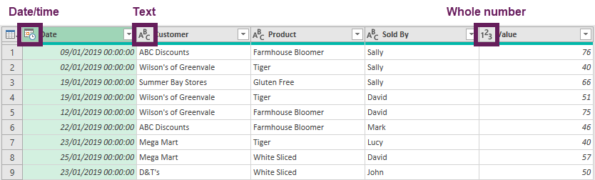
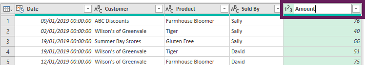
Double click on the “Value” column and change the name to “Amount”.

Next, click on the Date/Time icon and change it to a Date.

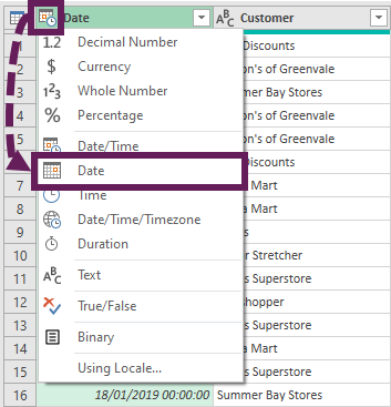
The Date column will now show the date icon, not the date and time icon.

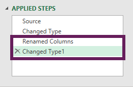
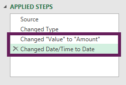
Look at the Applied Steps window; two new steps are added for our actions.

Take a look at the code in the Advanced Editor again. We can now see the code Power Query created for the additional transformations.

Editing the steps

We can click on the X symbol next to the name to delete a step. We can also right-click on a step to see all the editing options available.

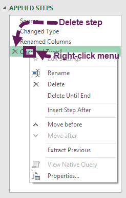
These options are generally self-explanatory. If there are any you don’t understand, then just try them out on some sample data… what’s the worst that’s going to happen 😀

Rename is probably the most useful command in here and the most underused. As the applied steps list gets longer, it can be challenging to remember what each step does. Therefore, it is good practice to rename steps when queries go beyond a few steps (see the screenshot below).

Load the data into Excel

To complete the process. We load the data back into the Excel workbook.

Click Home > Close & Load (drop-down) > Close & Load To… (note: clicking Home > Close & Load will apply your default settings).

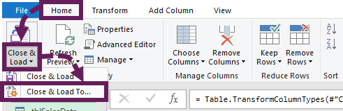
The Import Data dialog box opens. Select the options to load the data to a Table on New Worksheet, then click OK.

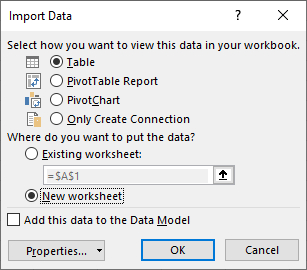
A new worksheet will be created, with a Table showing the transformed data.

You’re probably not blown away yet. All we have done is load a Table from Excel into Power Query, made a few minor changes, then loaded that data back into Excel. Remember, this is a simple example to show you the basic tool operations. As we move through this series, we will turn these simple steps into something amazing… I promise.

Importing data from Standard ranges

We can also import data from a standard range into Power Query. For example, if we selected a normal range (e.g., Cells A4:E54) and clicked Data > From Table/Range, before importing, Excel will automatically change those cells into a Table. Everything else after that point is identical to the steps above.

It is worth noting that this process will convert the range into a Table even if you don’t want it to. Excel will also apply a default Table name for you, so it may be called “Table1”, which isn’t particularly useful. However, as we’ve seen above, if we rename our Table later, we can change the name in the source step of the query too.

Importing data from named ranges

There is another way to tell Power Query the data range to import; by using named ranges.

The following uses Example 2 – Named Range.xlsx from the downloads.

The easiest way to create a named range is to select all the cells, then type the name into the Name Box and press Return.

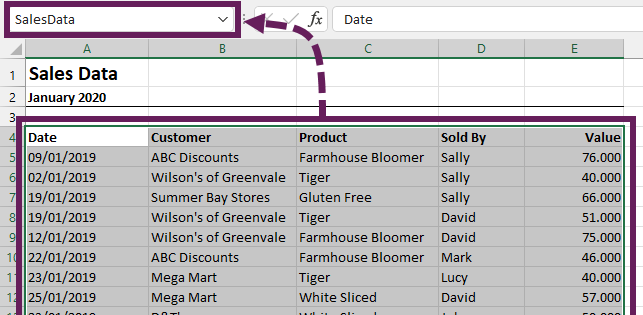
In the example file, a named range called SalesData has already been created.

Let’s import the data from the named range into Power Query. The steps are similar to importing data from a Table, so I will not repeat all the information from above, but I will highlight the differences.

Select the named range from the Name Box drop-down list. The range of cells will be selected on the worksheet.

Click Data > From Table/Range from the ribbon.

The data imported will look similar to when using a Table. However, there may be an additional applied step.

In this example, Excel adds an additional step of Promote Headers automatically. Click through the applied steps to see what changes have been applied.

The gear icon

Did you notice the small gear icon next to the Promoted Headers step? This is to indicate where Power Query allows us to change settings.

Click on the gear icon.

The Use First Row as Headers window will open. The window that opens will differ depending on the transformation step.

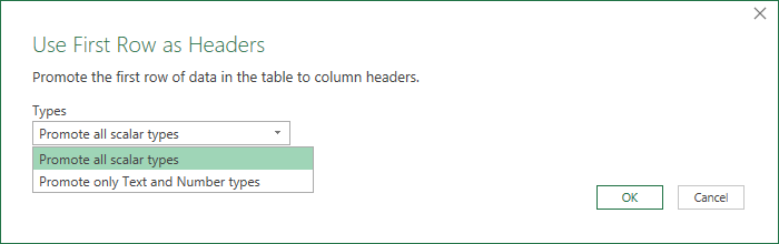
In our example, we still want the Promote all scalar types option; therefore, we can click OK without making any changes.

Display the Formula Bar

Rather than looking at all the M code in the Advanced Editor as we did before, we can view the code on a step-by-step basis in the Formula Bar.

If the formula bar is not visible, click View > Formula Bar

As we click through the steps, the formula bar changes, showing the M code used for each step. Initially, we do not need to worry about functions as the user interface is excellent. As we become more experienced, you will pick up a few functions and changes along the way.

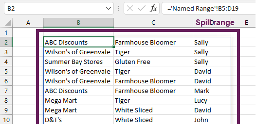
Importing data from dynamic arrays

If you have a dynamic array-enabled version of Excel (Microsoft 365 & 2021 later), this can be used as the source of the query.

Click on the first cell in the spill range. This will surround the spill range with a blue box. Click Data > From Table/Range to load the data into Power Query.

In the background, Excel:

• creates a named range linked to the spill range
• creates a query based on that named range

As the query is based on a named range, everything else continues the same as any other query based on a named range.

At this point, it is worth noting that Excel has created a named range for us, and therefore the name may not be very useful, it is likely to be something like “FromArray_1”. If we renamed the named range, we need to head back into Power Query and edit the source step in either the Advanced Editor or Formula bar.

Is it better to use named ranges or Tables?

Having looked at two options, named ranges and Tables, which is the best? Unfortunately, there is no straightforward answer, as it depends on your source data and scenario.

Tables

• Can auto-expand as new data is added to the bottom or right of the Table.
• Must be in a structured data format
• Must have a single defined header row
• Cannot have calculations in the header row

Named ranges

• Do not auto-expand as new data is added. Therefore, we may need to resize the named range as new data is added.
• Can contain any number of header rows (though it will require more transformations in Power Query)
• Can have calculations in the header row

Dynamic named ranges can be imported into Power Query too; that is outside the scope of this introduction.

My advice is to always opt for a Table, unless there is a specific reason not to.

Importing data from external files and Excel workbooks

Having looked at data stored in the same workbook as the query, let’s turn our attention to data stored outside the workbook.

Often, we open CSV files, text files, or Excel workbooks to copy and paste the data into another workbook. By importing the data directly into the workbook using Power Query, we never need to copy and paste again! The link to the source data is maintained and can be refreshed with the click of a button (more on that in the next post).

CSV File

CSV is a very common file format for exports from other systems. The good news is that Power Query loves CSV files.

The following uses Example 3 – CSV.csv from the downloads.

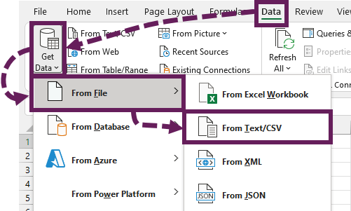
Start with a new workbook. Click Data > Get Data > From File > From Text/CSV

The Import Data window opens. Navigate to the CSV file, select it and click Import. Power Query opens a new window and displays a data sample.

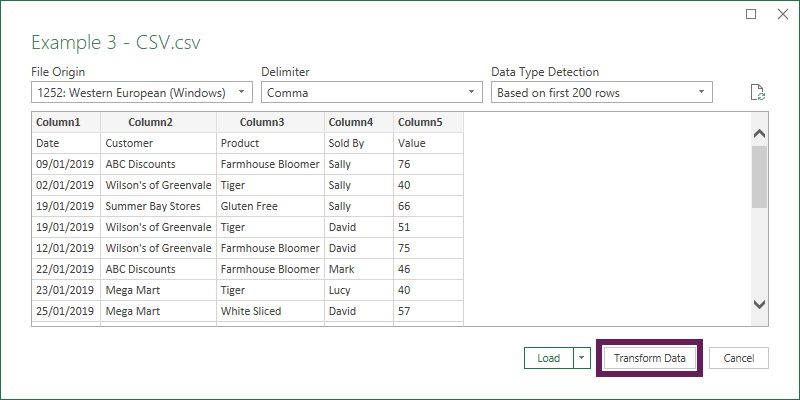
CSV files by definition have a comma delimiter, so there should be no need to change any of these settings.

To load the data directly into Excel without any changes we can click Load, but I do not advise this. We always want to see what our data looks like, so it is better to click the Transform Data button. All steps from now on are similar to what we have seen in the sections above.

Load data into Excel

Once the data is in Power Query, we follow the same steps as noted above to load that data as a Table into an Excel workbook. There are other destinations we can load the data to, and we will look at the most popular of these in future posts.

Text File

Text files are similar to CSV but can have a wider variety of data formats. Let’s look at a Tab delimited Text file to show how it is different.

The following uses Example 4 – Text.txt from the downloads.

Follow the same steps as for a CSV file. However, instead of selecting comma as the delimiter, Tab is likely to be selected by default. Depending on the file type, there are more options to choose from in the delimiter drop-down box.

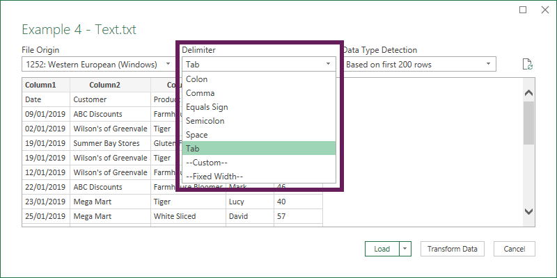
If the data you are importing is in another text format, select the appropriate option from the drop-down list. Then, click Transform Data to load the data into Power Query.

Excel workbook sheets

Finally, for this section, we will import the contents of an Excel workbook.

The following uses Example 5 – Excel Workbook.xlsx from the download.

Click Data > Get Data > From File > Excel Workbook. Navigate to your Excel workbook in the Import Data window and click Import.

The Power Query Navigator window opens. CSV and Text files contain a single source. An Excel workbook is different; it can have multiple worksheets, all of which are treated as separate data objects.

For this example, select the January worksheet and click Transform Data. We will be looking at combining multiple files in a future post.

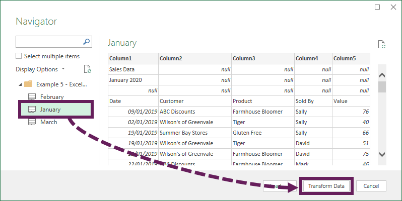
We are now presented with a scenario we have not encountered before. But it is a scenario that can occur in many circumstances – Excel doesn’t know which row contains the headers. Look at the screenshot below, Excel has assumed that row 1 of the spreadsheet contains the headers. But the headers should be Date, Customer, Product, Sold By, and Value, which are in row 3.

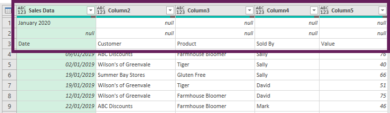
But don’t worry, we can fix this quickly with some simple transformations.

Let’s remove the top 2 rows. Click Home > Remove Rows > Remove Top Rows. The Remove Top Rows window opens. End 2 into the number of rows field, then click OK.

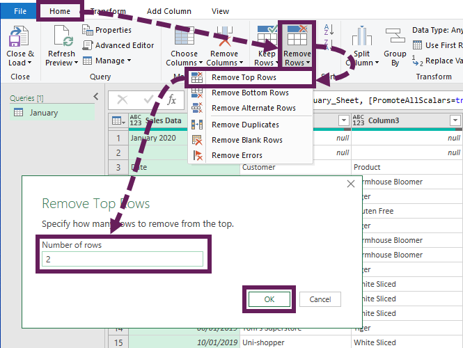
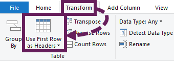
Next, we promote the new top row to be the header row by clicking Transform > Use First Row as Headers (note: the same transformation is also available in Home > Use First Row as Headers).

That’s it. We now have the same data format as the previous examples.

Wrap-up

This post shows us how to load data into Power Query using common sources – CSV, Text, Workbooks, Tables, and Ranges. For many users, these are the only data sources they will ever need to use. Through Power Query’s import and load process, we can eradicate many copy and paste actions previously used.

---

Read more posts in the Introduction to Power Query series

1. Introduction to Power Query
2. Get data into Power Query – 5 common data sources
3. DataRefresh Power Query in Excel: 4 ways  &  advanced options
4. Use the Power Query editor to update queries
5. Get to know Power Query Close & Load options
6. Power Query Parameters: 3 methods
7. Common Power Query transformations (50+ powerful transformations explained)
8. Power Query Append: Quickly combine many queries into 1
9. Get data from folder in Power Query: combine files quickly
10. List files in a folder & subfolders with Power Query
11. How to get data from the Current Workbook with Power Query
12. How to unpivot in Excel using Power Query (3 ways)
13. Power Query: Lookup value in another table with merge
14. How to change source data location in Power Query (7 ways)
15. Power Query formulas (how to use them and pitfalls to avoid)
16. Power Query If statement: nested ifs & multiple conditions
17. How to use Power Query Group By to summarize data
18. How to use Power Query Custom Functions
19. Power Query – Common Errors & How to Fix Them
20. Power Query – Tips and Tricks

---

What next?

Discover how you can automate your work with our Excel courses and tools.