How to unpivot in Excel using Power Query (3 ways)

Preparing data is probably the number 1 critical success factor in all data analysis and reporting. If the data layout is wrong, you’ll constantly be fighting Excel; You will have to use very advanced formulas; You will use unnecessary columns and might even duplicate data. Therefore, learning how to unpivot in Excel using Power Query is one of the most important skills you can have.

I used to be amazed at people who could use complex formulas. I picked up lots of tips and tricks by learning these advanced techniques. But I soon discovered that getting data in the correct format at the start meant I didn’t need those advanced formula skills. Because once the data is in the proper structure, Excel becomes easy.

This post shows you how to get the data into the correct structure by unpivoting in Excel using Power Query.

Table of Contents

What does it mean to unpivot your data?
Why unpivot in Excel?
Basic unpivot in Power Query
Unpivot with multiple columns
Unpivot with multiple header rows
Conclusion

Download the example file: Join the free Insiders Program and gain access to the example file used for this post.

File name: 0110 Unpivot data.xlsx

Get access

Now get Excel fired up and open the example file. We are ready to go!

Watch the video

&amp;amp;lt;span data-mce-type=”bookmark” style=”display: inline-block; width: 0px; overflow: hidden; line-height: 0;” class=”mce_SELRES_start”>&amp;amp;lt;/span>&amp;amp;lt;span data-mce-type=”bookmark” style=”display: inline-block; width: 0px; overflow: hidden; line-height: 0;” class=”mce_SELRES_start”>&amp;amp;lt;/span>&amp;amp;lt;span data-mce-type=”bookmark” style=”display: inline-block; width: 0px; overflow: hidden; line-height: 0;” class=”mce_SELRES_start”>&amp;amp;lt;/span>
Watch the video on YouTube.

What does it mean to unpivot your data?

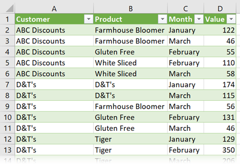
We often get information with categorization across the columns. Look at the example below.

We can see January, February, and March are in separate columns. But those columns are categorizations of the same type of data. So, a better layout would be to have a separate column for each month.

To process of moving the data from columns to rows is called unpivoting. Depending on who you speak to, it may be referred to as flattening or normalizing data.

Before Power Query, it took huge effort to transform data; we had to resort to formula complexity or long VBA codes. But Power Query has many features to make this transformation easy.

Why unpivot in Excel?

In the introduction, we said unpivoted data makes Excel easier to work with. You might be wondering why? Why bother to unpivot data in Excel at all.

Unpivoting changes your input from an informational/presentational layout into a data layout, which is efficient for computers to use.

Having a computer-optimized format makes it:

Easier to analyze data as we can pivot by any category
Easier to create visualizations as any category can be on an axis
Faster to calculate large volumes of data

Ultimately it comes down to this: unpivoted data is the ideal format for working with PivotTables, PivotCharts, formulas, and the Data Model. So, let’s aim to get our data into that format.

Basic unpivot in Power Query

Over three examples, we will progress from easy to tricky data layouts. But it will become clear that a grounding in a few basic transformations used in the right way is all it takes.

For our first attempt at pivoting data, we are using the Example 1 worksheet.

The source data displays a separate column for each month. However, rather than having a column for each month, it is better to have a column containing the month name as an attribute and a single value column.

Select any cell in the data range and change it into an Excel Table by clicking Insert > Table (or pressing Ctrl + T)

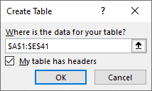
The Create Table window guesses the data range and if there is a header row. Since our data has a single header row, we can select the My table has headers option, then click OK.

Create Table dialog box recognizes headers

Give the Table a meaningful name (I have gone for tblSalesData).

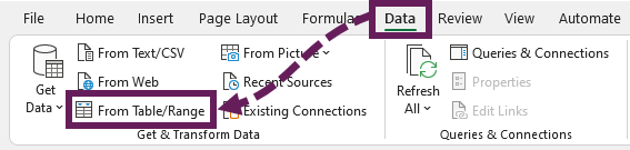
Now we are ready to load the tblSalesData Table into Power Query. Select a cell in the Table and click Data > From Table/Range.

The Power Query Editor opens, showing a preview of the data.

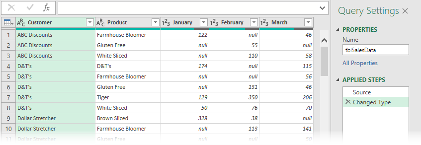
Delete the Change Type step. This step hardcodes the column headers into the M code, so it will break if we get new columns in our dataset.

OK, now let’s find out how to unpivot data.

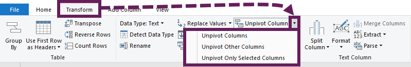
There are three options within the Transform > Unpivot Columns (drop-down) button. The option we choose depends on the outcome we want.

From those three options, there are only two outcomes:

Unpivot on the selected column
Unpivot on the unselected columns.

What is the difference, and is it important?

If we select the January, February, and March columns, and then apply the Unpivot Only Selected Columns, it would unpivot on those columns. Power Query creates a new column entitled Attributes containing months.

The M code to achieve this transformation would be:

= Table.Unpivot(#"Changed Type", {"January", "February", "March"}, "Attribute", "Value")

The column headers of January, February, and March are hardcoded into the M code. What happens if we add additional data for April? Power Query will not unpivot the new April column as it is not included in the code. But if you’re likely to add a new attribute column (for example, Size), it will work fine.

Instead, we could select the Customer and Product columns and use Unpivot Other Columns. For our current dataset, it achieves the same visual result in the Preview Window, but the M code in the formula bar is different.

= Table.UnpivotOtherColumns(#"Changed Type", {"Customer", "Product"}, "Attribute", "Value")

The code does not reference the month columns. Therefore, if we add any additional months into the source data, those months will also be unpivoted. This is great for data columns, but not attribute/dimension columns.

As in our scenario, we are more likely to get more months added, so Unpivot Other Columns is the best option.

Now, let’s tidy up the query with the following transformations:

Change the header of the Attribute column to Months.
Change the data type of each column to match the data within the column.

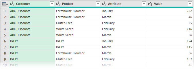
Click Close & Load to push the data into Excel. The worksheet will look like this:

From this, we can easily use formulas or PivotTables to create any view we want. This is the power that unpivoting our data gives us.

Unpivot with multiple columns

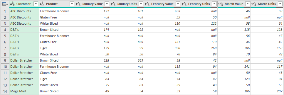
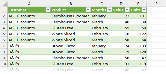
Now it’s time for Example 2. The source data looks like this:

Multiple columns of different data to unpivot

Instead of one column for each month, we now have two, showing sales Values and sales Units.

The most useful format is to have the month names in a single column with the Value and Units as separate columns.

The initial steps are the same as in Example 1:

Convert the data into a Table (use the first row as the header and exclude the total from the range).
Give the Table a meaningful name.
Click Data > From Table/Range to load the data into Power Query.
Just to be safe, delete any Change Type steps, which were created by Power Query automatically.

The Preview Window should be as follows:

Multiple column data in Power Query to unpivot

Select the Customer and Product columns and click Transform > Unpivot Columns (drop down) > Unpivot Other Columns

Now we need to make quite a few transformations; these depend on your specific dataset. So, the instructions below might not match your exact scenario.

At this stage, our data is over-normalized. We have Values and Units in the same column, but these are different data units.

Over normalized data with values and units in same column

We need to pivot back to separate the Values and Units.

Select the Attribute column, and split the column into the parts we need.
For our example, we need to split by the space character. Click Transform > Split Column > Split by Delimiter, then apply the settings in the image below.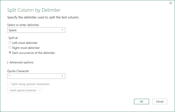
The Attribute column is split into two separate columns.
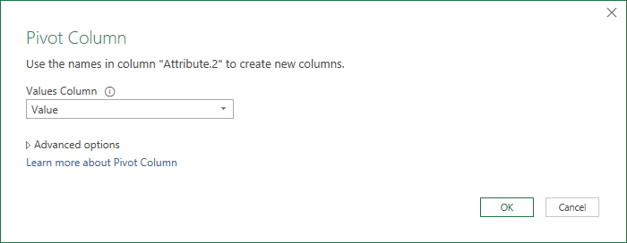
Select the column which displays Values and Units (probably called Attribute.2), then click Transform > Pivot Column. In the Pivot Column window, select the column containing the numbers, then click OK.
Change the names of the Attributes.1 column to Months.
Set the data type for each column.

Finally, click Close & Load to push the data into Excel.

The unpivoted data in Excel now looks like this:

Perfect!

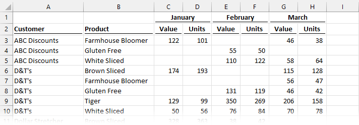
Unpivot with multiple header rows

It’s now time for our final example. Everything is the same as in Example 2, except for the table headers. We have two header rows, the first showing Months and the second showing Value or Units.

Unpivot in Excel with muliple header rows

Separating the headers into multiple rows is a presentational format that is very difficult to work with.

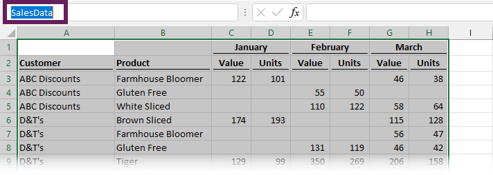
Excel Tables can only have a single header row. Since we have two header rows, let’s use a named range instead of a Table.

Select the entire range and enter the name SalesData into the name box.

Named Range used to get data into Power Query

Then, with the named range selected, click Data > From Table/Range.

After the data has loaded into Power Query, remove any automatically applied steps such as Promoted Headers and Changed Type. We just want the Source step.

The Preview Window shows the following:

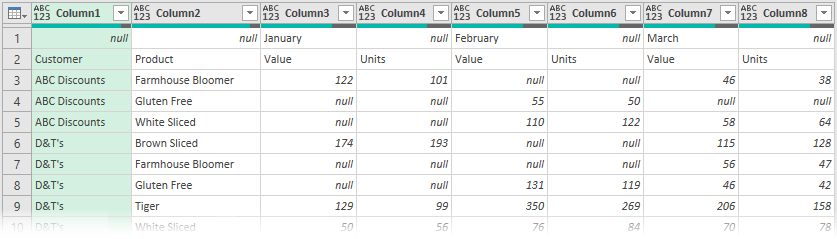
Multi column data to unpivot loaded into Power Query

This view gives us a problem; it doesn’t show the month in every column. If we try to unpivot, it will unpivot the null value. So, we first need to use the Fill Across transformation… but wait… there isn’t one!

Instead, we transpose the data, apply the Fill Down transformation, then transpose it back again.

Click Transform > Transpose
Select Column1, click Transform > Fill (drop-down) > Down
Select Column1 and Column2
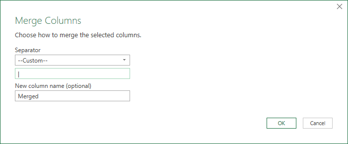
Click Transform > Merge Columns
In the Merge Columns window, choose a separator that is not in the text of the two columns already (I have selected for a pipe ( | ))
Click Transform > Transpose to return the data back to its previous format
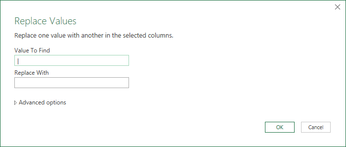
Select Column 1 and Column 2.
Click Transform > Replace Values. Replace the | with [blank]. This removes the | character from the Customer and Product columns we added in a previous step
Now promote the first row as the header by clicking Transform > Use First Row as Headers

After all those transformations, the Preview Window will look like this:

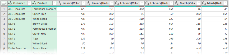
Data with multiple column headers combined into a single column

It’s now a similar format as we had in Example 2. So, to complete this example, follow through with all the transformation steps from example 2.

Conclusion

Learning to unpivot in Excel is critical to your ability to work efficiently. If the data is in the correct layout, it is easy to work with and avoids complexity. Power Query gives us the tools to unpivot data in various situations.

Read more posts in this series