Refresh Power Query in Excel: 4 ways + advanced options

Previously, we looked at how to import data from various file formats and load it into Excel using Power Query. In this post, we move on to consider how to refresh that data. Refreshing data is important as it enables us to build a query once and use it over and over (that is automation in action).

Table of Contents

• Refresh Power Query
• Create a basic query
• Simple transformations
• Refresh the query
• Using VBA for refresh all
• Refresh specific queries
• Refresh button
• Queries & connections menus
• VBA refresh
• Advanced refresh options
• Power Query refresh in Excel Online
• Wrap-up

The download includes 2 files:

• Example 6 – Data Refresh 1.csv
• Example 6 – Data Refresh 2.csv

Refresh Power Query

Unlike Excel’s calculation engine, which by default re-calculates with every worksheet change, Power Query only recalculates when specifically told to.

The basic refresh process is straightforward, click Data > Refresh All. However, there are lots of options to customize the refresh, and optimize it for your scenario. We look at the refresh options later in this post also.

The following examples, use Example 6 – Data Refresh 1.csv and Example 6 – Data Refresh 2.csv from the downloads.

Create a basic query

To demonstrate the data refresh capabilities of Power Query we first need to create a query.

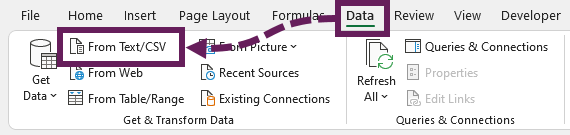
To work along with the example, open a new workbook and click Data > From Text/CSV (also available under Data> Get Data > From File > From Text/CSV).

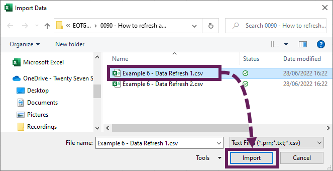
The Import Data window opens. Navigate to Example 6 – Data Refresh 1.csv, select it and click Import.

A new dialog box opens and displays a sample of the data. Click Transform Data.

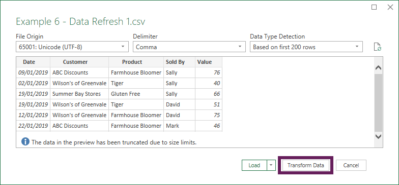
This loads the sample data into the preview window.

Simple transformations

We will now make some simply data transformations to shape the CSV into useful information. This is the first time in this series we are performing some of these transformations, so it’s a good idea to follow along and get an understanding of the user interface. We will definitely be using these transformations again in the future.

Delete the Changed Type step

The first step to undertake is deleting the Changed Type step by clicking on the cross next to the step.

There are specific issues with dates in Power Query. The CSV file has UK date format of dd/mm/yyyy, but if your region does not accept that date format it may result in errors for you. Therefore, we delet the auto applied Changed Type step which may cause this issue.

Apply date based on Locale

To get a valid date format for your region:

• Click on the ABC icon in the header of the Date column
• From the menu select Using Locale….
• In the Change Type with local dialog box apply the following:
  • Data Type: Date
  • Locale: English (United Kingdom)

Click OK.

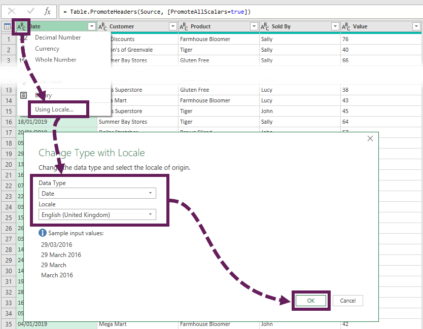
This tells Power Query that the column contains a UK date format.

Change data types

Now, let’s re-apply the default data type for the remaining columns. Click Customer, hold the Shift key and click Value. Then, click Transform > Detect Data Type from the ribbon.

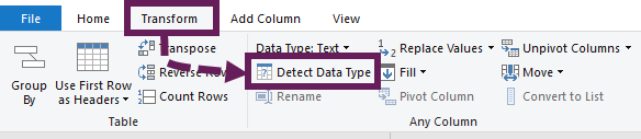
Power Query should now have the correct data types for every column.

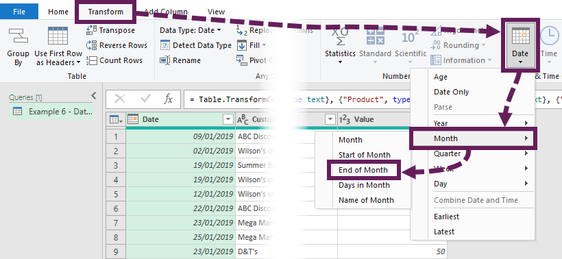
Change date to month end date

We are creating a report based on month-end dates, so let’s change the date. Click on the Date column. From the ribbon, click Transform > Date > Month > End of Month (this will change the Date column to the last day in the calendar month).

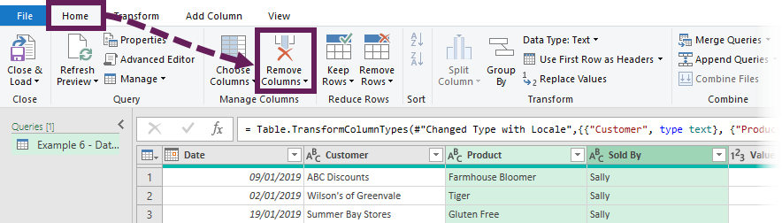
Remove columns

There are two columns we don’t need for our example. Select the Product and Sold By columns. From the ribbon click Home > Remove Columns (this removes the selected columns).

Pivot the data

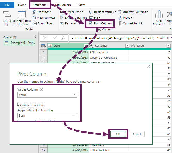
Now let’s pivot on the data. Select the Date column and click Transform > Pivot Column.

The Pivot Column dialog opens. Apply the following settings:

• Change the Values Column to Value (this is column to be aggregated)
• In the advanced options section set the Aggregate Value Function to Sum
• Click OK

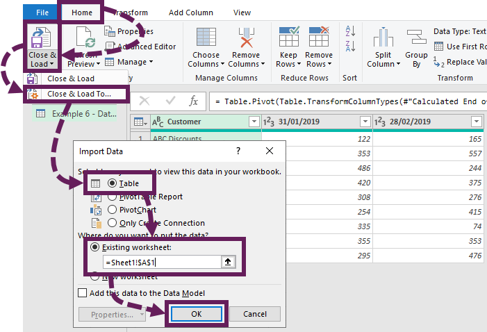
Finally, click Home > Close & Load (drop-down) > Close & Load To…

Then, in the Import Data dialog box select a Table on a new worksheet, click OK.

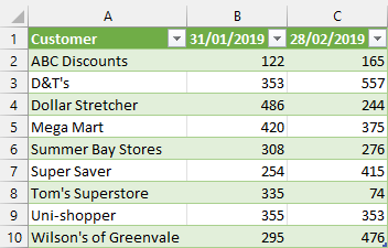
Excel creates a new worksheet with a report containing the customer sales for January and February. This table contains the data from the CSV, which has been transformed. It should look like the screenshot below.

Refresh the query

To demonstrate the refresh process, we are simulating where a user might receive a new file on a daily, weekly, or monthly basis.

• Delete the Example 6 – Data Refresh 1.csv file
• Rename the Example 6 – Data Refresh 2.csv file to Example 6 – Data Refresh 1.csv

When we refresh, Power Query looks for a file called Example 6 – Data Refresh 1.csv. It doesn’t know it is a different file. In fact, we don’t want Power Query to know it’s been replaced, we just want it to process what is there.

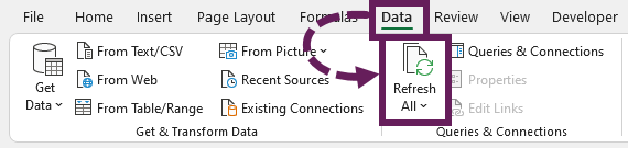
Click Data > Refresh All.

In the background, Excel imports the data from the CSV file, the same transformations are applied, and the data is loaded into the worksheet as a Table.

The new data should appear automatically on the worksheet.

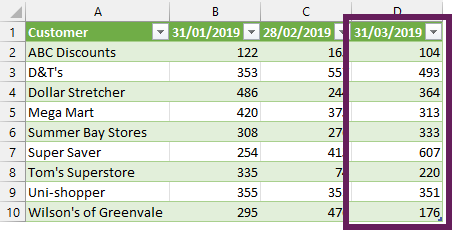
Did you notice the March data appeared with a single click,  that is amazing!

Each time there is a change to the existing data, or when a new file is received, it is only necessary to save the file with the same file path, then click one button. That is powerful stuff… right?

In a future post, we will look at linking the file path to a cell, so you can import without having to rename any files.

Using VBA for refresh all

The VBA code to refresh all queries is the same as refreshing all PivotTables. Enter the code snippet below into a standard VBA code module.

Sub RefreshAll()
ActiveWorkbook.RefreshAll
End Sub

If we attach this macro to a shape or form control button, we create a simple user interface for anybody using our workbook to refresh queries.

Refresh specific queries

When we have lots of queries within a workbook, it can take a while to refresh them all. In these circumstances, it may useful to refresh only the queries we need. There are a few ways to achieve this.

Refresh button

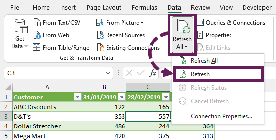
If you click on a Table, which comes from a query, we can click Data > Refresh All (drop-down) > Refresh to refresh only that specific query.

Queries & connections menus

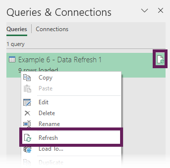
When loading the data from Power Query into Excel, the Queries and Connections menu opened. This window shows all the queries created in the workbook. If that menu is not open, click Data > Queries and Connections

Each query listed in Queries and Connection has a refresh icon. Simply click the icon to refresh the data for that query.  Alternatively, we can right-click on the query and select Refresh from the menu.

VBA refresh

With a VBA macro, we can refresh individual queries. The code snippet below refreshes the Example 6 – Data Refresh 1 query.

Sub RefreshQuery()
ActiveWorkbook.Connections("Query - Example 6 - Data Refresh 1").Refresh
End Sub

This is a useful technique when:

• we want to provide an easy-to-use interface for the user
• we want to control the query refresh order

Advanced refresh options

As more queries are added to a workbook, it can soon become time-consuming to refresh individual queries, or too slow to refresh them all. The good news is that Excel already has advanced options to control refresh.

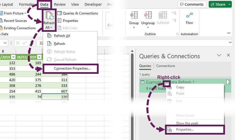
Select a cell within a query Table, then click Data > Refresh All (Drop Down) > Connection Properties. Or right-click on the query in the Queries and Connections pane and click Properties…

The Query Properties window opens.

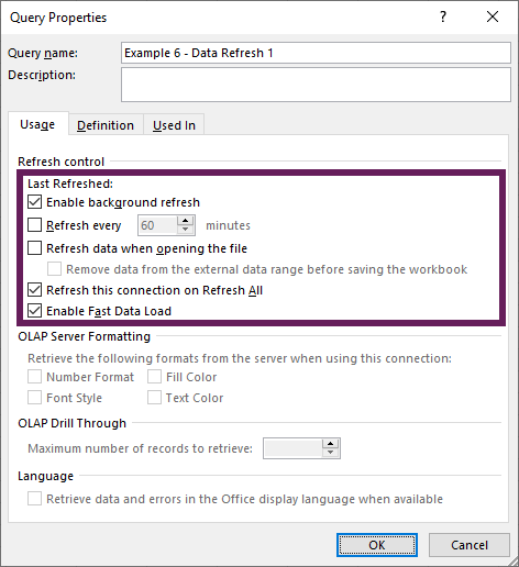
The important refresh options available in this window are:

Background refresh – This allows us to keep working while the data refreshes in the background. It is turned on by default. If we remove this option, we are unable to use Excel until the refresh process completes.

This option has bigger consequences though. If we have background refresh enabled:

• PivotTables refresh before Power Query. This is a problem if our PivotTable is based on a query; it means we must click refresh twice.
• Macros may execute before the query refresh has completed.

If background refresh is disabled, the refresh occurs in the correct order; PivotTables update and VBA macros execute after the query has refreshed. While it might lock up Excel for a short period of time, it is better to know the data is correct. Generally, I recommend disabling background refresh for all queries.

Refresh every x minutes – This option controls how often a query is refreshed. This only operates if the workbook is open. It is useful when the source data is regularly changing. It is probably a good idea only to use this option with the background refresh enabled, or it could become very annoying for users to wait for Excel to update on a regular basis.

Refresh when opening the file – Automatically refreshing data when opening the file is a useful feature as you know the data is up-to-date whenever you open the file.

Refresh this connection on Refresh All – Where a query contains static data, there is no need to refresh it every time. By disabling the Refresh this connection on Refresh All option, it removes these queries from the Refresh All process, which in turn, reduces the refresh time.

Enable Fast Data Load – We all want data to load faster, right? So why would you not click the Enable Fast Data Load option? Well… it may make Excel lockup for periods of time on loading, but it will make the data load faster. A study by Andrew Moss indicated that time savings for Fast Data load were 18%-33%. Personally, I always want the most up-to-date data, so recommend having this checked.

Power Query refresh in Excel Online

At the time of writing, Microsoft has started making progress with bringing Power Query to Excel Online. At present we can only refresh a small number of data sources:

• From Table/Range
• From Anonymous OData Feeds

There is still a long way to go before Power Query is fully available in Excel online.

Find more info here: https://techcommunity.microsoft.com/t5/excel-blog/new-in-excel-for-the-web-power-query-refresh-is-now-generally/ba-p/3300369

Wrap-up

This post shows us how to refresh Power Query. When refreshing, data is re-imported and follows the same transformation steps. Through this, Power query enables us to automate all of these steps down to a single click.

---

Read more posts in the Introduction to Power Query series

1. Introduction to Power Query
2. Get data into Power Query – 5 common data sources
3. DataRefresh Power Query in Excel: 4 ways  &  advanced options
4. Use the Power Query editor to update queries
5. Get to know Power Query Close & Load options
6. Power Query Parameters: 3 methods
7. Common Power Query transformations (50+ powerful transformations explained)
8. Power Query Append: Quickly combine many queries into 1
9. Get data from folder in Power Query: combine files quickly
10. List files in a folder & subfolders with Power Query
11. How to get data from the Current Workbook with Power Query
12. How to unpivot in Excel using Power Query (3 ways)
13. Power Query: Lookup value in another table with merge
14. How to change source data location in Power Query (7 ways)
15. Power Query formulas (how to use them and pitfalls to avoid)
16. Power Query If statement: nested ifs & multiple conditions
17. How to use Power Query Group By to summarize data
18. How to use Power Query Custom Functions
19. Power Query – Common Errors & How to Fix Them
20. Power Query – Tips and Tricks

---

What next?

Discover how you can automate your work with our Excel courses and tools.