Power Query Append: Quickly combine many queries into 1

Data doesn’t always come in one single file, or from one download. Therefore, we have to find a way to stitch multiple files together so we can use it as if it were a single data source. This might be cost center reports, monthly data extracts, product profiles, survey data, etc. Basically, it applies to any data which comes from multiple sources. To combine these sources, we use the Power Query append transformation.

The Power Query append transformation allows us to combine queries of a similar column layout into a single query. Also, don’t forget we refresh all the data sources with a single click of Data > Refresh All. By using the append transformation, we can put an end to tedious copy and paste routines for combining multiple files.

If you are looking to combine data sources by looking up values from source, you need the merge transformation. Find information about the merge transformation here.

Table of Contents

Scenario
Create the first query
Duplicate and edit the query
Append queries
Append another query
When column headers are different
Combining files of different types/data structures

Download the example file: Join the free Insiders Program and gain access to the example file used for this post.

File name: 0104 Power Query Append.zip

Get access

The examples in this post use the following files:

January 2019.xlsx
February 2019.xlsx
March 2019.xlsx
April 2019.xlsx

We will work through all the steps from start to finish, so get Excel fired up, and let’s get going.

Watch the video

Watch the video on YouTube.

Scenario

The example we are working through combines multiple periods of sales data into a single query.

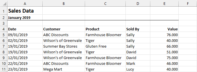
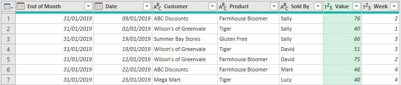
The screenshot below shows the first rows from the January 2019.xlsx file. The other files follow a similar column structure.

In reality, we would be unlikely to use this approach for this type of scenario. As the source data has a consistent layout, we are more likely to combine all the files in a folder. We tend to use the append transformation when data comes from sources of inconsistent layout (e.g., A financial nominal ledger report and a budget spreadsheet). Then, we reshape each data source individually before combining them into a single query. However, to demonstrate the technique, this approach will work fine.

Create the first query

Open a new Excel workbook; this will be where the combined data will be loaded.

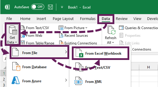
Click Data > Get Data > From File > From Workbook.

Navigate to the January 2019.xlsx file from the downloads and click Import.

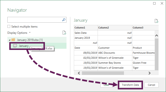
From the Navigator window, select the workbook containing the data (the January worksheet in our example), then click Transform Data.

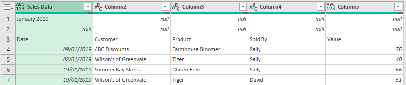
The Power Query editor will open, showing a Preview of the data.

Note: For this example, I assume the default settings are applied inside Power Query. Therefore the Promoted Headers and Changed Type steps are implemented automatically.

We need a few simple transformations to get this into a usable format.

Remove the top two rows by clicking Home > Remove Rows > Remove Top Rows. Enter 2 into the Remove Top Rows window and click OK.
Promote the first row of data to the header by clicking Transform > Use First Row as Headers
Add a month-end date column by selecting the Date column, then click Add Column > Date > Month > End of Month
With the Date column still selected, add a week number column by clicking Add Column > Date > Week > Week of Year
Rename the Week of Year column to Week
Move the End of Month column to the start by Right-clicking on the End of Month column header and select Move > To Beginning from the menu.
Check the following data types have been applied; if not, apply them manually.
- End of Month = Date
- Date = Date
- Customer = Text
- Product = Text
- Sold By = Text
- Value = Whole Number
- Week = Whole Number

After the transformation steps above, the preview window should look like this:

Power Query Preview Window after changes

That’s all the transformations we need for now. Let’s load this as a Connection Only.

Click Home > Close and Load To… from the ribbon.

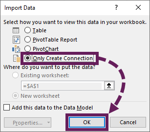
In the Import Data dialog box, select Only Create Connection, then click OK.

Only Create Connection for the source queries

The Queries & Connection pane shows only the January query (click Data > Queries & Connections from the ribbon if this pane is not visible in Excel). Nothing is loaded to the worksheet.

Queries & Connections window displaying query with Connection Only

Duplicate and edit the query

For our example, we don’t want to go through the same transformation steps again. So instead, we will duplicate the January query, then change the steps to work with the February.xlsx file.

Open the Power Query editor by double-clicking on the January query in the Queries & Connections pane.

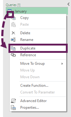
In Power Query, right-click on the January query in the Queries pane and select Duplicate.

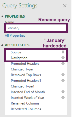
In the Query Settings pane, rename the duplicate query to February.

The first two steps of our example have hardcoded “January” within the M code, so we must edit these steps. Therefore, we need to change any references from January to February. How you edit these steps is up to you. Either click the settings icon, next to the step, or edit the M code directly in the Formula Bar or Advanced Editor.

Query Settings pane - rename query + highlight hardcoded steps v2

In terms of the M code, the changes are as follows:

Source:

= Excel.Workbook(File.Contents("C:\Users\marks\Power Query Examples\January 2019.xlsx"), null, true)

Becomes:

= Excel.Workbook(File.Contents("C:\Users\marks\Power Query Examples\February 2019.xlsx"), null, true)

Navigation:

= Source{[Item="January",Kind="Sheet"]}[Data]

Becomes:

= Source{[Item="February",Kind="Sheet"]}[Data]

That’s it. Click Close and Load To… to load the February query as Create Connection Only.

The Queries and Connections will now show the January and February queries.

Append queries

The Power Query append transformation is reasonably straightforward.

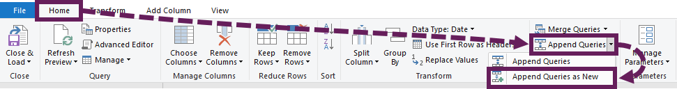
Open the Power Query editor. Then, click Home > Append Queries (drop down) > Append Queries As New

The Append dialog box opens. There are two views possible in this dialog box:

View for combining two queries
View for combining three or more queries

Both views are straightforward to use, as shown below.

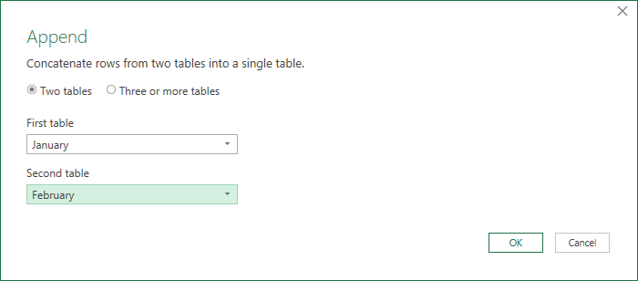
View for combining two queries

In this view, select the two queries to be combined from the drop-down boxes. The Primary table always appears first in the combined query.

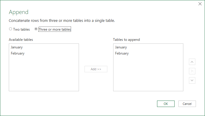
View for combining three or more queries.

In this view, select the queries in the left pane and click Add to move them into the list of tables to append.

From either view, after clicking OK, a new query is created. As shown below, both queries are now combined into a single Table.

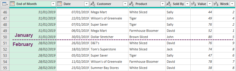
The query is probably given a default name of Append1; make sure you give it a more meaningful name, such as Combined Sales Data.

The M code function which combines the tables is Table.Combine. Find out more about this function here: https://learn.microsoft.com/en-us/powerquery-m/table-combine

Click Close and Load to load the query into a new worksheet as a Table.

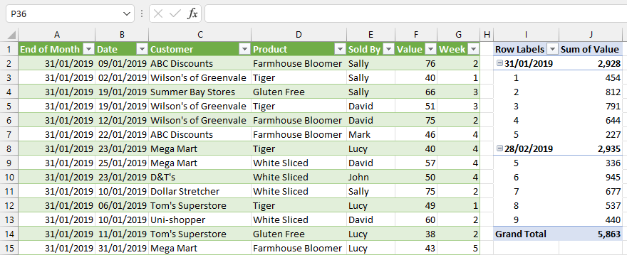
Take a look at the new Table in Excel. It contains both January & February data. To illustrate this, I added a Pivot Table showing the End of Month, Week and Values.

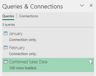
There are now three queries within the workbook; January, February, and Combined Sales Data.

Append another query

Next, try adding the March 2019.xlsx file on your own. Follow the same steps above to create the connection, then edit the combined query to include the March data. You must use the three or more tables option in the Append dialog box.

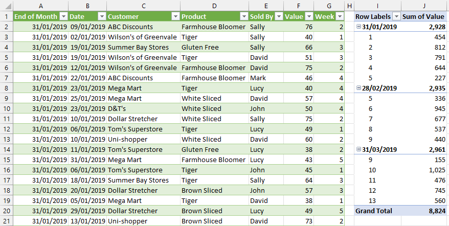
After adding March, the data and Pivot Table look like this:

Got it? That all seems relatively straightforward, doesn’t it?

When column headers are different

Now let’s look at the April.xlsx file. It is slightly different from the others; the Customers column header has changed to Sold To. These small changes happen regularly when dealing with manual data sources. Unfortunately, others make tweaks to the files without realizing it impacts our process.

If we follow the same steps above, the query breaks at any actions where the Customers column header is hard coded within the M code.

Power Query can’t find a column called Customer. As we know, Customers column is now called Sold To in the source file.

For this example, we will take a simple approach. Click through the steps from top to bottom; each time you identify a step causing the error, update the M code in the Formula Bar to refer to Sold To rather than Customer.

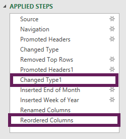
If the error occurs on a Changed Type step, change this code:

= Table.TransformColumnTypes(#"Promoted Headers1",{{"Date", type date},
    {"Customer", type text}, {"Product", type text}, {"Sold By", type text}, {"Value", Int64.Type}})

To this:

= Table.TransformColumnTypes(#"Promoted Headers1",{{"Date", type date},
    {"Sold To", type text}, {"Product", type text}, {"Sold By", type text}, {"Value", Int64.Type}})

If the error occurs on the Reordered Columns step, change this:

= Table.ReorderColumns(#"Renamed Columns",{"End of Month", "Date",
    "Customer", "Product", "Sold By", "Value", "Week"})

To this:

= Table.ReorderColumns(#"Renamed Columns",{"End of Month", "Date",
  "Sold To", "Product", "Sold By", "Value", "Week"})

After applying the changes above, the query should be working again.

Follow the instructions above to add the April query to the Combined Sales Data query.

There is still a problem. Look at the screenshot below.

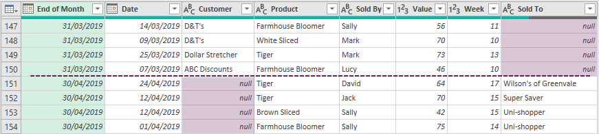
Data Problem caused by different column names

The Customer and Sold To columns were both the 3rd column in the relevant queries, yet they appear as two separate columns.

This is a crucial point to note. Power Query uses the column headers to determine which columns to combine, not the position within the query.

We need to give the queries consistent column headings. In the April query Rename the Sold To column header to Customer.

Now the columns should combine correctly.

Close and Load the data back into Excel. April is the only new query, so load this as a Connection Only.

Combining files of different types/data structures

We saw above that when appending queries, columns with the same column header combine into the same column. Therefore, we can combine data from any sources into one query provided we give them the same column headings.

Where all the files have a consistent structure, we can automate this further by combining all the files in a folder.

Microsoft’s documentation about the Power Query append transformation can be found here: https://support.microsoft.com/en-us/office/append-queries-power-query-e42ca582-4f62-4a43-b37f-99e2b2a4813a

Read more posts in this series