In this post, we use Power Query to import all the files in a folder. We give Power Query a folder path, click a few buttons, and it imports and combines all the files into a single table. It’s like magic!
To add another file to the output table, we only have to save a copy of the file in the folder and click refresh; the new file will be imported too. This can save us days of time over a month.
Before we get started on this technique, there is one point to make you aware of. The files to be imported must follow a similar structure and column pattern. Power Query is magic, but you’ve got to give it a reasonable chance. There are more advanced techniques we can use to combine files with different structures, but that is not for the faint-hearted and is outside the scope of this post.
The most common file types for Excel users are CSV and Excel workbooks. So, these are the two file types covered in this post. If you have other files, such as .txt, XML or JSON, etc., you can still use the techniques in this post, but it will require some changes to the process.
Table of Contents
Download the example file: Join the free Insiders Program and gain access to the example file used for this post.
File name: 0107 Power Query Combeind Files.zip
The examples in this post use the following files:
CSV Files:
- January 2019.csv
- February 2019.csv
- March 2019.csv
- April 2019.csv
Excel Workbooks:
- January 2019.xlsx
- February 2019.xlsx
- March 2019.xlsx
- April 2019.xlsx
Watch the video

Setting up the example
To work along with the example in this post, start by moving the January and February files into a separate folder (both the .csv and .xlsx files). These are the files to import initially.
In the example, I have used a folder called Import Folder.
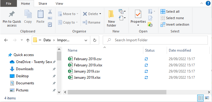
Do not include the March or April files in the folder at this stage. We will add those files later as part of the example.
Combine all CSV files in a folder
The easiest files to combine are CSV or text files, so that’s where we will start.
What makes CSV files easy to work with?
- They always contain a single table
- The first row is treated as the header row
- Merged cells are not permitted
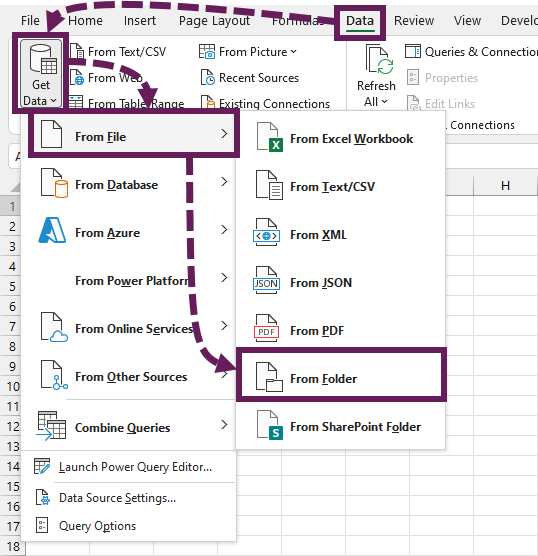
In Excel, click Data > Get Data > From File > From Folder
Navigate to the folder containing the files to import, then click Open.
A preview of the folder and file attributes is displayed.
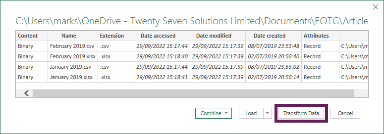
If the files are uniform and no edits are required, we could click Combine (drop-down button) > Combine Close & Load. However, you’ll notice we have a mix of .csv and .xlsx files in the folder; we can’t combine these easily. Instead, we click Transform Data and take a closer look at what’s happening here.
My advice is always to click Transform Data to ensure the data is correct before pushing it into Excel.
The Power Query editor opens. However, it does not show the data from the files as we might be used to seeing. Instead, Power Query shows data about the files. This is the same process used to list the files in a folder.
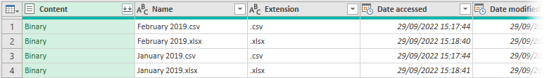
Our first transformation keeps only the files we wish to be combined (i.e., the CSV files for our current example). It is good practice to filter to only include the files we need; you never know when another user might decide to save a random file type within the folder.
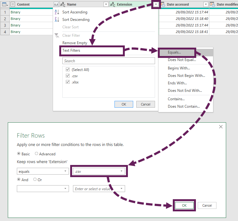
First, change the file extension to all lowercase. With the Extension column selected, click Transform > Format > lowercase. As Power Query is case sensitive, this step ensures that .CSV and .csv are treated the same. While we don’t have an issue with our example files, it is good to future-proof where we can.
Next, filter the Extension column to include only .csv. Click Filter > Text Filters > Contains… . In the Filter Rows dialog box, enter .csv, then click OK. Again, this step future-proofs; it ensures any non-CSV files are excluded.
From here, we have a two options
- Combine the files
- Use a Custom Column to extract the data for each file
Technically, there are other options, but they are more advanced than we are looking at in this post. Which method you choose is up to you. You may even decide to use different methods for different circumstances.
Method 1: Combine files
Method 1 uses Power Query’s magic built-in combine process.
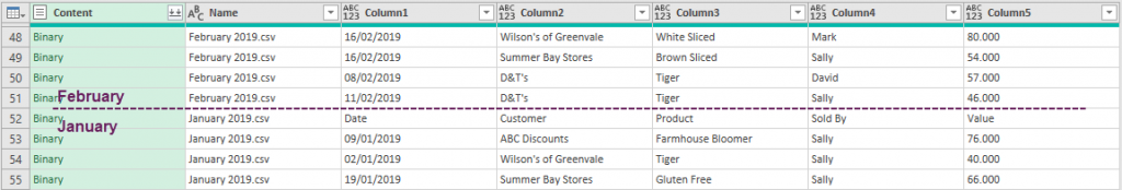
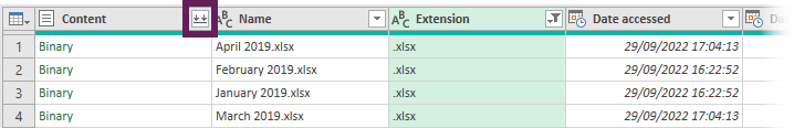
The Preview window should currently look like this:

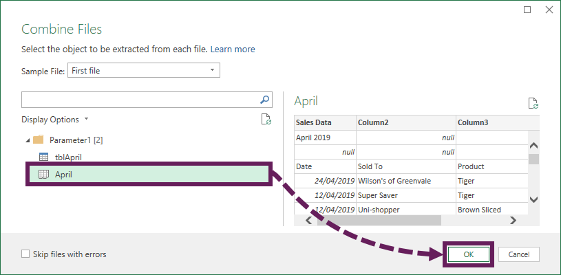
Did you notice the icon with the two down arrows at the top of the Content column? That’s the Combine Files icon. If we click the icon, Power Query creates a lot of queries and steps for us. Effectively it drills from the file level into the content level and combines each file.
Go ahead and click the Combine Files icon… you know you want to.
The Combine File window opens, showing a sample of the data using the first file in the query as an example.
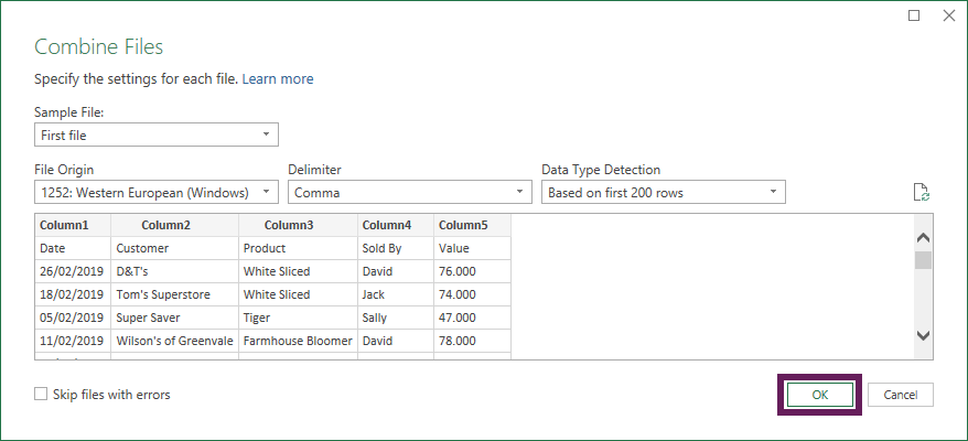
You may wonder why the first file has February instead of January dates. This is because February comes before January alphabetically.
All looks good, so click OK.
Power Query now does its magic. Once it has finished, we see the files are combined. That’s all it took, one button!
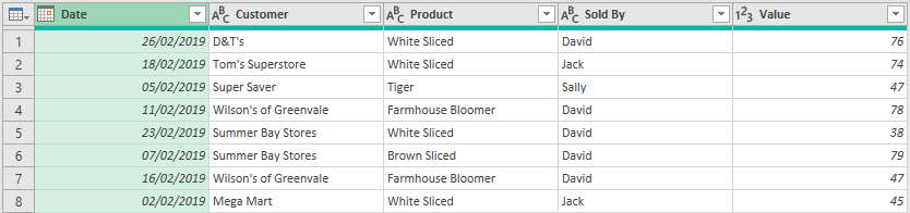
The preview data should look like this:
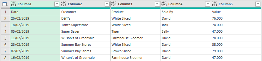
If you scroll down, you see that the January and February data are combined into a single table.
In the background, Power Query creates a lot of transformations to achieve this (see the highlighted sections below)
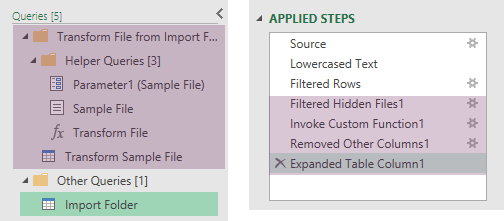
What’s going on with all these queries?
You may wonder what all these files do. As a quick summary:
- Parameter1 – A parameter to hold the file name of the selected sample file.
- Sample File – A file object of the selected sample file.
- Transform File – A custom function applied to every file in the folder. The steps in the function are based on the Transform Sample File query.
- Transform Sample File – A query that contains the transformations applied to Sample File. Forms the basis of the Transform File custom function.
- Import Folder (or whatever yours is called) – This is the final query with all the files stacked together.
There are two locations we can make transformations:
- Transform Sample File – All transformations made in this query are applied to all files in the folder
- Main query (the Import Folder in my example) – This is a combined query, so all transformations apply to the combined data.
We should try to perform any changes to our data in the Transform Sample File first.
With the Transform Sample File query selected:
- Promote headers by clicking Home > Use First Row As Headers
- Change the data type for each column. Be aware, the dates in the CSV file are in UK date format, so you may need to select Using Locale… > Date > English United Kingdom for the date column.
The transformations are applied to every file in the folder and combined into the Import Folder query.
Unfortunately, the data types do not get pulled into the main query. So, we need to reapply the data types in the main query.
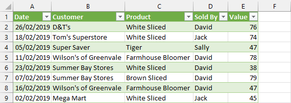
Finally, click Home > Close & Load to load the data into Excel.
Method 2: Use a Custom Column
The second method uses a Custom Column containing the Csv.Document Power Query function.
Follow the steps from Method 1 to load the data into Power Query. The preview window should look like this:
Next, let’s start making transformations.
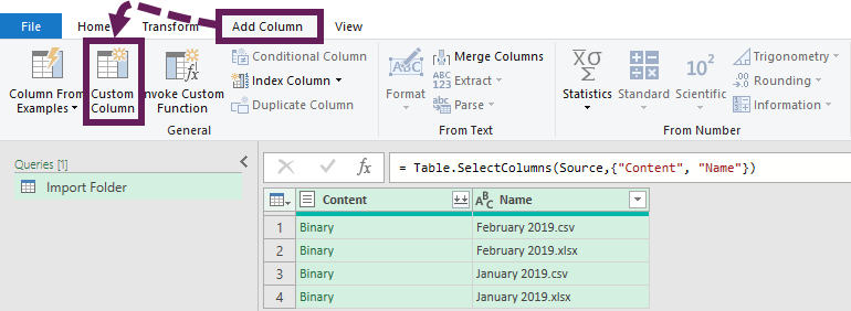
Select the Content and Name columns, then click Home > Remove Columns > Remove Other Columns. This removes the columns which we do not require.
Click Add Column > Custom Column.
In the Custom Column window, input the following information
New column name: CSV
Custom column formula:
=Csv.Document([Content])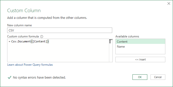
Click OK to execute the function.
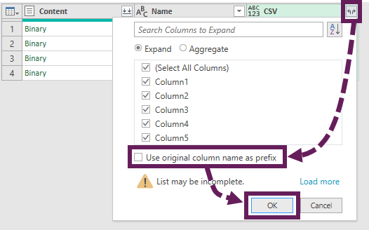
A new column called CSV is added to the preview window. The name is based on the text entered into the Custom Column dialog box.
You will notice a new double arrow icon in the CSV column header. This is the Expand icon and indicates that the column contains more detail that we can drill into.
Click on the Expand icon. Uncheck the use original column name as prefix option, then click OK.
We now have the data from both files combined into a single view.
Files are stacked on top of each other, similar to an append transformation.
To tidy up everything, we need to undertake some more transformation:
- Select the Content and Name columns and click Home > Remove Column
- Promote headers by clicking Home > Use First Row As Headers
- In the Date column, filter to remove the text value “Date”
- Set the data types for each column. Remember, the dates are in a UK format, so you may need to use Using Locale… > Date > English United Kingdom.
Our preview window should now look like this:
That’s it, all done. Click Close & Load to load the data into Excel. The January & February files are combined.
Adding more files to the folder
Now it’s time to add more files to the folder. Copy the March 2019.csv file into the folder.
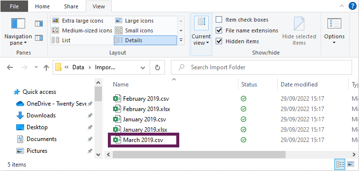
Now for the moment of truth… in Excel, click Data > Refresh All.
The table updates with the new data from March. Don’t tell me you’re not impressed. It’s amazing!!!!
File uniformity is the key to success
Now add the April 2019.csv file into the folder. Then, click Data > Refresh All.
We get an error:

Why did this happen? What went wrong?
Open up April 2019.csv and take a close look at the first row. All other files had Customer in Cell B1, but April has Sold To.
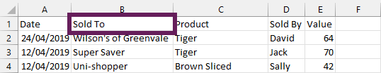
This was to illustrate the importance of having consistent column headers. We could employ other advanced methods to avoid this error; however, the best option is to ensure consistent headings.
Combine Excel workbooks in a folder
The method to import Excel workbooks is similar to CSV files. But as Excel workbooks contain multiple sheets, and those sheets can have almost any name, there is additional complexity.
Power Query likes to hardcode values into the query M code. This becomes a problem when Excel workbooks have worksheets with different names.
To test us, all our Example files in our example have different worksheet names.
Copy the March 2019.xlsx and April 2019.xlsx files into the folder.
In Excel, follow these steps (similar to the previous examples)
- Click Data > Get Data > From File > From Folder
- Navigate to the folder, then click Open
- When the list of files appears, click the Transform Data button
- The Power Query Editor window opens
- With the Extension column selected:
- Transform to be only lower case
- Filter to include only .xlsx files
Let’s look at the same two methods we used above.
Method 1: Combine files
Method 1 uses Power Query’s built-in combine process. After the previous steps, the preview window should look like this:
Next, click the Combine icon as before.
As April.xlsx is first in the list of files alphabetically, Power Query will use this as a sample file. On the Combine Files window, select the April sheet and click OK.
As you might expect, only the April data loads correctly into the Preview window for our scenario. There is only one workbook with a worksheet called April, so only one worksheet loads correctly. We must find the location in the M code where the sheet name has been hardcoded and adjust it.
Open the Transform Sample File query and click on the Navigation step in the applied steps pane.
The M code for this step looks like this:
= Source{[Item="April",Kind="Sheet"]}[Data]
This tells us that a filter is applied for Items called “April,” where the object type is a Sheet. Delete the item name. The M code should now be this:
= Source{[Kind="Sheet"]}[Data]
Go back to the main query and look at the Preview window again. All the worksheets are now combined – that’s magic!
Let’s finish the transformations. In the Transform Sample File:
- Remove the top 3 rows by clicking Home > Remove Rows > Remove Top Rows
- Promote the first row to a header by clicking Transform > Use First Row as Headers
- Apply the correct data types to each column.
Head back to the main query and make any changes so the query works correctly (you will likely need to delete and reapply the Changed Type step).
Method 2 – Use a Custom Column
Method 2 uses a Custom Column formula, similar to the CSV example above. However, this time the formula applied is Excel.Workbook.
Assuming we hadn’t undertaken Method 1. Follow the same steps until the Preview Window looks like this:
Select the Content and Name columns, then click Home > Remove Other Columns.
Now let’s add the new column; click Add Column > Custom Column.
In the Custom Column window, input the following information:
New column name: ExcelFile
Custom column formula:
=Excel.Workbook([Content])
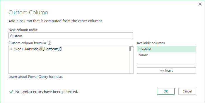
Click OK.
A new ExcelFile column is added. Click on the double arrow Expand icon, uncheck the option to use original column name as prefix, then click OK to include all the columns.
Every worksheet and table from the workbook is listed.
The April file contains worksheets and tables. Filter the Kind column to include only sheets.

Select the Data column, then click Home > Remove Other Columns.
Click the Expand icon on the Data column to drill down into the data.
We now have all the sheets combined into a single query.
Let’s make some transformations to tidy things up.
- Remove the top 3 rows by clicking Home > Remove Rows > Remove Top Rows
- Promote the first row as the header by clicking Transform > Use First Row as Headers
- Apply the correct data types to each column.
- Filter the Sold By column to remove the values null and SoldBy
Finally, Close and Load the query into Excel.
Ta-dah! All is good in the world once again.
Notes & tips
Here are a few bonus tips:
- When looking for files, Power Query will look in sub-folders too. This is great when files are organized within a defined structure. But if the folders are in a mess, then some housekeeping might be required to get this method to work. Or you could edit the M code to change Folder.Files to Folder.Contents.
- Plan for what might go wrong. Think about what might happen if somebody else were to save a different file type in the folder. When you create the query, include extra filter steps to ensure only the files you want are imported.
- Data that comes from an IT system usually works well with this technique. Unfortunately, I find that any data generated by user input tends to cause problems. Because people like to change things, they add columns; they rename sheets, and they type over static values. So, if your files come from user input, be prepared to use some advanced transformations. In this scenario, the append transformation will be useful.
Read more posts in this series
- Introduction to Power Query
- Get data into Power Query – 5 common data sources
- DataRefresh Power Query in Excel: 4 ways & advanced options
- Use the Power Query editor to update queries
- Get to know Power Query Close & Load options
- Power Query Parameters: 3 methods
- Common Power Query transformations (50+ powerful transformations explained)
- Power Query Append: Quickly combine many queries into 1
- Get data from folder in Power Query: combine files quickly
- List files in a folder & subfolders with Power Query
- How to get data from the Current Workbook with Power Query
- How to unpivot in Excel using Power Query (3 ways)
- Power Query: Lookup value in another table with merge
- How to change source data location in Power Query (7 ways)
- Power Query formulas (how to use them and pitfalls to avoid)
- Power Query If statement: nested ifs & multiple conditions
- How to use Power Query Group By to summarize data
- How to use Power Query Custom Functions
- Power Query – Common Errors & How to Fix Them
- Power Query – Tips and Tricks
Discover how you can automate your work with our Excel courses and tools.
The Excel Academy

Make working late a thing of the past.
The Excel Academy is Excel training for professionals who want to save time.