How to Interpolate in Excel: 4 simple ways

Interpolation is the process of estimating data points within an existing data set.  As this is an Excel blog, then clearly the question we want to answer is: can we interpolate with Excel.  This is a common question.  In fact, it was the following question from a reader which first made me look into this topic:

“I have an Excel question – Is there a way to interpolate a value from a table?  I have an X and Y that are not on the table, but have correlated data so want to calculate the interpolated value”.

As a simple example, if it took 15 minutes to walk 1 mile on Monday and 1 hour to walk 4 miles on Tuesday, we could reasonably estimate it would take 30 minutes to walk 2 miles.

This is not to be confused with extrapolation, which estimates values outside of the data set.  To estimate that it would take 2 hours to walk 8 miles would be extrapolation as the estimate is outside of the known values.

Excel is an excellent tool for interpolation, as ultimately, it is a big visual calculator.

Table of Contents

• Options for interpolation with Excel
• Interpolation using simple mathematics
• Interpolation using the FORECAST function
• Interpolation when perfectly linear
• Interpolation when approximately linear
• Interpolation when the data is not linear
• Interpolate exponential data
• Inner linear interpolation
• Conclusion

Watch the video

Watch the video on YouTube.

Options for interpolation with Excel

In terms of answering the question, there are several scenarios that would lead to different solutions.

Firstly, we could just use simple mathematics.  This would work if the results were perfectly linear (i.e., the X and Y values move directly in sync with each other).  But if they are not, we could have a slightly skewed result.

Alternatively, we could use Excel’s FORECAST function (or FORECAST.LINEAR in Excel 2016 and beyond). Based on its name, the FORECAST function seems like an odd choice.  It would appear to be a function specifically for extrapolation; however, it is also one of the best options for linear interpolation in Excel.  FORECAST uses all the values in the dataset to estimate the result; therefore it is excellent for linear relationships, even if they are not perfectly correlated.

Then another thought, what if the X and Y relationship is not linear at all?  How could we interpolate a value when the data is exponential?

Let’s take a look at all these scenarios.

Interpolation using simple mathematics

Simple mathematics works well when there are just two pairs of numbers or where the relationship between X & Y is perfectly linear.

Here is a basic example (look at the Example 1 tab in the supporting download file):

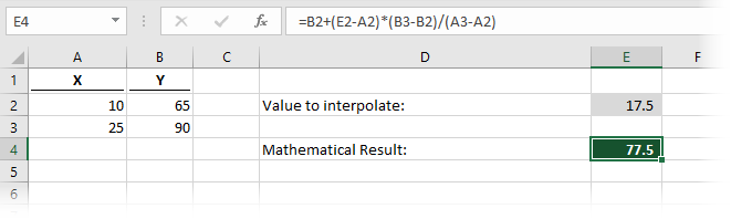
The formula in cell E4 is:

=B2+(E2-A2)*(B3-B2)/(A3-A2)

That might look a bit complicated to some, so here is a quick overview of the formula.

=B2+(E2-A2)*(B3-B2)/(A3-A2)

The last section (highlighted in green above) calculates how much the Y value moves whenever the X value moves by 1.  In our example, Y moves by 1.67 for every 1 of X.

=B2+(E2-A2)*(B3-B2)/(A3-A2)

The second section (in green above) calculates how far the interpolated X is away from the first X, then multiplies by the value calculated above.  Based on our example, the result calculates as 17.5 (cell E2) minus 10 (cell A2), the result of which is then multiplied by 1.67.  This all equals 12.5.

=B2+(E2-A2)*(B3-B2)/(A3-A2)

Finally, we get to the first section of the formula (in green above), which is adding the first Y value.  In our example, this provides the final result of 77.5 (65 + 12.5).   For anybody who remembers high school mathematics, the formula is as follows:

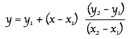
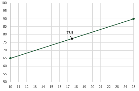
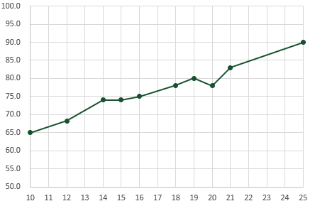
Here is the result overlaid onto a chart.

Even if you don’t remember linear interpolation that from school, the good news is that Excel has given us a more straightforward option, the FORECAST function.

Interpolation using the FORECAST function

In the 2016 version of Excel, there were lots of new statistical functions added.  To make room for these new functions, FORECAST has been replaced with the FORECAST.LINEAR function.  Though FORECAST still remains at the moment for the purpose of backward compatibility with Excel 2013 and before.

As FORECAST and FORECAST.LINEAR are effectively the same, we’ll be using the terms interchangeably.

Interpolation when perfectly linear

Now let’s use FORECAST to interpolate a result.

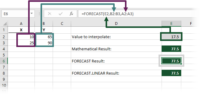
Using the same numbers from the example above, the formula in cell E6 is:

=FORECAST(E2,B2:B3,A2:A3)

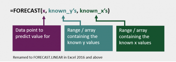
The FORECAST function has the following syntax:

=FORECAST(x,known_y's,known_x's)

The three arguments in the function are:

• x – the data point for which we want to predict a value
• known_y’s – the range of cells or array of values containing the known Y values
• known_x’s – the range of cells or array of values containing the known X values

When using the FORECAST function, the result of cell E6 is also 77.5 (just as in the mathematical approach).

For completeness, the example file also contains the use of FORECAST.LINEAR function.  As we would expect, the result is identical to the legacy FORECAST function.

Interpolation when approximately linear

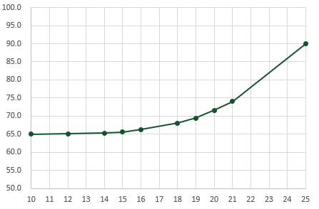
But… what if our data isn’t perfectly linear?  Look at the chart below, the data clearly has a linear relationship, but it’s not perfect.  Look at the Example 2 tab in the supporting file.

In these circumstances, the FORECAST function is even more useful, as it does not just interpolate between the first and last values.  Here is the data used in the chart.

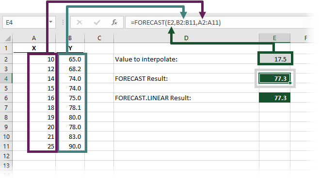
The FORECAST function in cell E4 interpolates the Y value based on the X value of 17.5.

=FORECAST(E2,B2:B11,A2:A11)

In this scenario, FORECAST estimates a value based on all the available data points, not just the start and end.  The result of the FORECAST function in cell E4 is 77.3 (rounded to 1 decimal place), which in most circumstances would be more accurate than the simple linear interpolation applied in the mathematical approach.

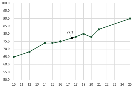
Remember, interpolation is used to estimate values.  77.3 may not be the exact result, but it is a reasonable estimate based on the information we have.

Once again, FORECAST.LINEAR calculates the same result.

Interpolation when the data is not linear

But, here’s a trickier question, what if the data is not linear at all?  Then what?

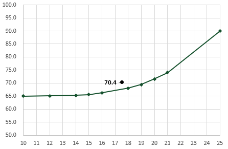
Look at the Example 3 tab in the supporting file.  Here is our new chart scenario:

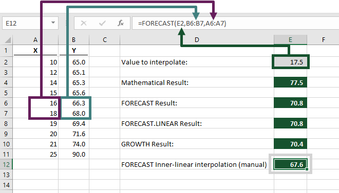
If we took a simple linear approach, that would give us a value of 77.5, which as you can see below, is quite a long way from the curve.  Using the FORECAST function would provide a result of 70.8, which is better, but also a long way from the curve.

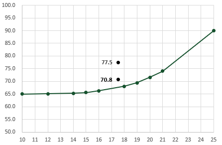
There are two further options to get a better estimate (1) interpolating exponential data using the GROWTH function (2) calculating an inner linear interpolation

Interpolate exponential data

The GROWTH function is similar to FORECAST but can be applied to data with exponential growth.

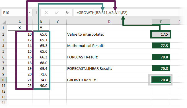
The result of the GROWTH function in cell E10 is 70.4.  Once again, this is closer to the line, but still a little way off.

The formula in cell E10 is:

=GROWTH(B2:B11,A2:A11,E2)

The GROWTH function has the following syntax:

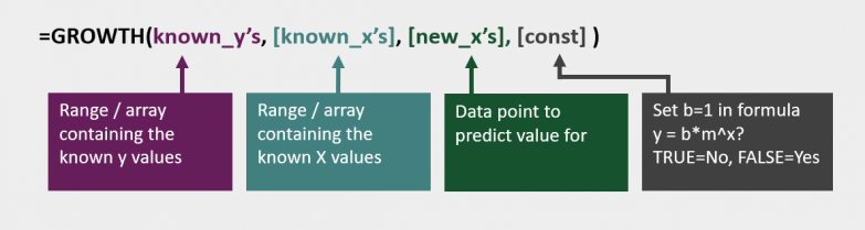
=GROWTH(known_y's,[known_x's],[new_x's],[const])

The four arguments in the GROWTH function are (just be aware the arguments are not in the same order as the FORECAST function).

• known_y’s – the range of cells or array of values containing the known Y values
• [known_x’s] – the range of cells or array of values containing the known X values
• [new_x’s] – the data point for which we want to predict a value
• [Const] – a true/false measure to indicate how the formula should calculate.  For our scenario, we can leave off this last argument.

The square brackets are to indicate which arguments are optional for the function to calculate a result.  We need the known_y’s, known_x’s, and new_x’s, but have ignored the const argument.

While the result of 70.4 is a closer approximation, we must not use the GROWTH function with blind faith.  Test your interpolations to check if they are reasonable.

Inner linear interpolation

A reasonable option may be to find the result above and below the new X value, then apply linear interpolation between those two points.  This would get pretty close.

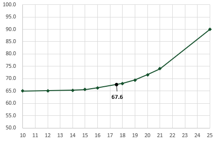
In our example, the values on both sides of an X of 17.5 are:

• X:16 and 18
• Y: 66.3 and 68

Using these values, we can now do a standard linear interpolation.

Quick, single-use method

If this were a one-off action, we could do this quickly by including only the essential cells in the formula.

=FORECAST(E2,B6:B7,A6:A7)

However, as soon as we change the interpolated value, FORECAST may calculate an inaccurate result.   So, let’s move on to look at a flexible method.

Flexible approach

To create a flexible approach, we will use the INDEX, MATCH, and FORECAST functions combined.  This may sound tricky, but don’t worry, we’ll walk through it slowly.  Ultimately we are trying to achieve the same result as the single-use method above, but automatically adjusting the ranges depending on the value being interpolated.

NOTE: For this method to work, it does require the range of known X’s to be listed in ascending order.

MATCH function

Firstly, we use the MATCH function to retrieve the position of the value lower than 17.5.

=MATCH(E2,A2:A11,1)

This formula is saying find the value in Cell E2 from the range of Cells A2-A11.  The 1 at the end of the formula tells the MATCH function that we wish to use an approximate match (i.e., the closest value below the lookup value).  16 is the closest value below 17.5.  As 16 is the 5th item in cells A2-A11, MATCH returns a value of 5.

INDEX function

Having identified in the previous stage that the 5th position contains the value below, we can use the INDEX function to determine the cell reference for this value.

INDEX(A2:A11,MATCH(E2,A2:A11,1))

This would return a reference to cell A6.

To find the value above, we can use the same function, but add 1 to the MATCH function.

INDEX(A2:A11,MATCH(E2,A2:A11,1)+1)

The formula above would return a reference to cell A7.

Dynamic range

Now things start to get interesting.  We can combine these functions with a colon ( : ) in the middle to create a range for the two X values.

INDEX(A2:A11,MATCH(E2,A2:A11,1)) : INDEX(A2:A11,MATCH(E2,A2:A11,1)+1)

The first INDEX function returns the reference to cell A6 (the result of the green highlighted section).  The second INDEX function returns the reference to cell A7 (the result of the purple highlighted section).  These are separated by a colon ( : ) (highlighted in red), to create a range – A6:A7

We can do the same to create a range for the two Y values.  The only difference is the INDEX functions will look at Cells B2-B11.

INDEX(B2:B11,MATCH(E2,A2:A11,1)) : INDEX(B2:B11,MATCH(E2,A2:A11,1)+1)

By using Cells B2-B11 in the INDEX function, it will calculate a range B6:B7.

INDEX MATCH & FORECAST

Now we have our two ranges; the X values A6:A7 and the Y values B6:B7.  Let’s combine all of this within the FORECAST function.

=FORECAST(E2,
INDEX(B2:B11,MATCH(E2,A2:A11,1)):INDEX(B2:B11,MATCH(E2,A2:A11,1)+1),
INDEX(A2:A11,MATCH(E2,A2:A11,1)):INDEX(A2:A11,MATCH(E2,A2:A11,1)+1))

That’s a pretty big formula, right.  But, hopefully I’ve managed to explain it so that it’s not too scary.

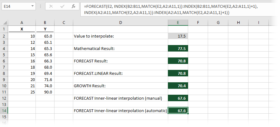
The result of the inner-linear interpolation using the FORECAST function is 67.6 (to 1 decimal place, shown in cell E14).  Have a look at the chart again; you will see that 67.6 is a reasonable estimation based on the data available.

WARNING: Ultimately, this is still a linear interpolation calculation based on the two values either side of the X value.  The distance between the values above and below will have a direct impact on how accurate the interpolation is.

Conclusion

Initially, what seemed like a simple question has lead us to lots of potential solutions for three different scenarios.  The key is that you need to know your data to select the method which provides the most accurate results.

In the process, we have covered the FORECAST and FORECAST.LINEAR functions and have seen that they are useful for interpolation as well as extrapolation.

Also, in this post, we have used INDEX and MATCH to create dynamic ranges, which is a very powerful technique for advanced formulas in Excel.

If you’re looking for further information about forecasting techniques in Excel, then check out Engineer Excel (https://engineerexcel.com/blog).  While you might not be working in an engineering context the techniques are applicable in many other circumstances.

---

What next?

Discover how you can automate your work with our Excel courses and tools.

The Excel Academy