In this post, we look at 6 easy ways to calculate how many days are between two dates using Microsoft Excel. As often with Excel, there are many ways to achieve a calculation, so we look at the most useful options for calculating days.
Dates can be tricky to work with as there are often weekends and public holidays to contend with. But don’t worry, we’ll also show you how to deal with those.
All the examples use UK date formats, but the principles apply no matter which format you use.
Table of Contents
How Excel treats dates
In Excel, dates are just normal numbers with a special format applied. Excel calculates dates based on the number of days since 31st December 1899:
- 1 January 1900 = 1
- 2 January 1900 = 2
- 3 January 1900 = 3
- 20 July 1969 (Moon landing) = 25374
- 1 January 2000 (Current Millenium) = 36526
Note: When Excel was developed, Lotus 1-2-3 was the dominant spreadsheet software. Unfortunately, Lotus 1-2-3 had a bug incorrectly treating 29th February 1900 as a valid date. As Excel had to supply the same calculation result as Lotus 1-2-3, this bug was purposefully included. Excel is now the dominant software, but correcting the bug would break too many existing spreadsheets, so the bug remains. Therefore, any days calculation that crosses 29th February 1900 may be incorrect by 1 day.
In Excel, to get a date from the date serial number, we format the number as a date. To do this:
- Click Home > Number Format launcher (or Press Ctrl + 1)
- In the Date category, we can select different locales and format types.
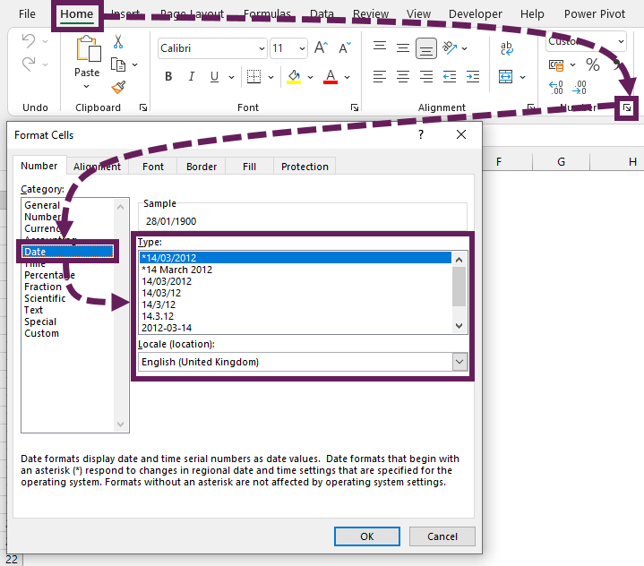
For more advanced date formatting, use a custom number format.
Decimal values are used to calculate time. For example, 25404.84514 is 8:17 pm on 20th July 1969. Use the INT function to remove the time element from a date. The formula below removes the decimal places and returns 25404, which can be a date serial number.
=INT(25404.84514)Convert text formatted dates to actual dates
Sometimes the date appears to be a serial number in a date format; instead, it is text that looks like a date. What should we do in these circumstances?
Provided the text is in a structure that Excel can understand as a date, then Excel is normally good at converting it automatically. However, even after this automatic conversion, we should check to ensure it is calculating correctly; we don’t want to get caught out by different country date formats.
Other times Excel won’t recognize the date format at all. This depends on regional settings. For example, in the UK, 14/04/2022 is converted to a date, even if it is text. Yet, 14.04.2022 is text that is never converted. However, in other countries, 14.04.2022 is converted to a date.
In these situations, the following solutions are useful:
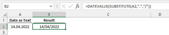
DATEVALUE & SUBSTITUTE function
The SUBSTITUTE function replaces specific characters in a text string; then, the DATEVALUE function ensures the text string is converted to a numeric value.
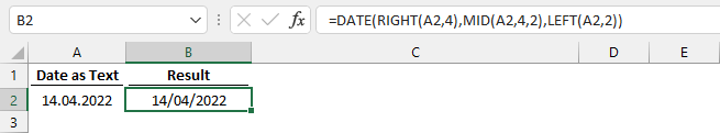
DATE, LEFT, MID & RIGHT functions
Or, as an alternative method, the DATE function is used.
DATE creates a valid date based on 3 arguments; Year, Month, and Day. The individual date elements are extracted from the text string using the LEFT, MID, and RIGHT Excel functions.
TODAY function in Excel
Often, we may wish one of the dates in our calculation to be the current date, or based on the current date. In this scenario, we use the TODAY function to return the serial number of the current date.
=TODAY()Enter the function above into a cell, or use it in a formula to get today’s date.
Rather than today, we may wish to have a relative date. An example of this would be calculating an invoice due date which is 30 days from today. For this, we add or subtract the number of days from the TODAY function. For example, the formula below calculates the date 30 days from today.
=TODAY() + 30
Subtract dates in Excel to get days
The simpliest method to calculate the number of days between dates is to subtract one date from another:
Look at the screenshot below. We can use a simple formula to calculate the number of days between 4th August 2022 and 13th September 2022.
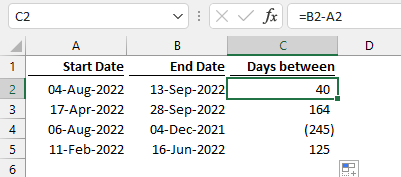
The formula in Cell C2 is Cell B2 minus Cell A2:
=B2-A240 is returned as the number of days between the dates.
In the example, I double-clicked the fill handle to copy the formulas down.
In the previous section, we detailed how Excel handles dates; therefore, this calculation is a simple subtraction of two date serial numbers.
Dealing with negative days
If we have negative values, it simply means the second date is later than the first. If you are only interested in days, irrespective of which came first, use the ABS function in Excel. The ABS function returns the absolute value (i.e., it ignores any negative signs).
In the screenshot below, all calculations return absolute values. The value in Cell C4, which is a negative number in the example above, is now positive.
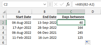
The formula in Cell C2 is:
=ABS(B2-A2)Include the start and end dates
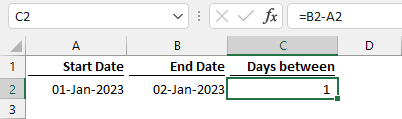
In Excel, dates start at midnight. Therefore, if you have to calculate the days between 1st January and 2nd January, it will return a result of 1, rather than 2.
When calculating dates, we often want to include the start and end date. To achieve this, we add 1 to the value
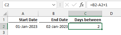
The formula in Cell C2 is:
=B2-A2+1Excel DAYS function
The DAYS function was introduced in Excel 2013 (for Windows, Excel 2011 for Mac); it is specifically designed to count the number of days between two dates.
Syntax
=DAYS (end_date, start_date)Arguments
- End_date – The end date as a serial number
- Start_date – The start date as a serial number
Look at the screenshot below. It calculates the same results as the above example, but using the DAYS function.
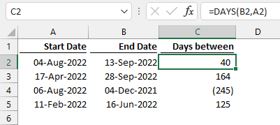
The formula in Cell C2 is:
=DAYS(B2,A2)Just like the earlier method, DAYS returns the number of days between two dates. Therefore, to include the start and end dates in the calculation, adjust the formula accordingly.
=DAYS(B2,A2) + 1Excel DATEDIF function
Another helpful Excel function for returning the number of days between two dates is the DATEDIF function.
The DATEDIF formula calculates the date difference between two dates over different time periods: number of days, number of months, or number of years.
DATEDIF was introduced in Excel to ensure compatibility with Lotus 1-2-3, but it has never really been accepted as a standard Excel function. It is not listed in Excel’s function library, and there are no tooltips to help write the formula. However, if we enter the formula using the syntax below, it provides the correct result.
Syntax
=DATEDIF(start_date,end_date,unit)Arguments
- Start_date – The start date as a serial number
- End_date – The end date as a serial number
- Unit – The time unit to use (years, months, or days)
- “Y” = Difference in days in full years
- “M” = Difference in days in full months
- “D” = Difference in days
- “MD” = Difference in days. Years and months are ignored
- “YM” = Difference in months. Years are ignored
- “YD” = Difference in days. Years are ignored
Look at the screenshot below. It uses the same values as before, but applies the DATEDIF function.
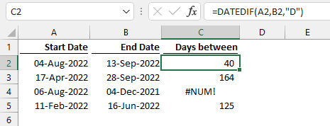
The formula in Cell C2 is:
=DATEDIF(A2,B2,"D")While DATEDIF returns the number of days between two dates, it does not work where the start date is after the end date. In these circumstances, DATEDIF returns the #NUM error (shown in Cell C4).
If we want to return another time frame, we can change the “D” in the third argument for another unit code (e.g., “M”, “Y”, “MD”, “YM”, “YD”). This argument must be in double quotes or a cell value.
Calculate working days between two dates
In many business situations, rather than the total number of days, we may need to exclude weekends and public holidays. For these situations, we use the NETWORKDAYS function.
Syntax
=NETWORKDAYS(start_date, end_date, [holidays])Arguments
- Start_date – The start date as a serial number
- End_date – The end date as a serial number
- Holidays Optional – a range of cells or an array containing a list of dates to exclude from the calculation
Without the last argument, the NETWORKDAYS function provides the number of days, excluding weekend days.
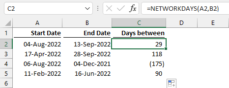
The formula in Cell C2 is:
=NETWORKDAYS(A2,B2)Additionally, if we provide a list of public holidays, they are also excluded from the calculation.
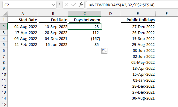
The formula in Cell C2 is:
=NETWORKDAYS(A2,B2,$E$2:$E$14)The dates in Cells E2-E14 are excluded from the final results. Therefore, this formula returns only the number of workdays (excluding weekends and holidays).
If your business days are not Monday to Friday, then check out the Excel NETWORKDAYS.INTL function, as it provides additional arguments to adjust the weekend days.
Power Query to subtract dates to calculate days
Now let’s move on to look at some Power Query options.
Once the data has loaded into Power Query, we need to ensure the start and end dates have the date data type applied; otherwise, the dates may not be recognized.
From there, we add a Custom Column by clicking Add Column > Custom Column. Then, we can enter the following formula:
=[End Date]-[Start Date]
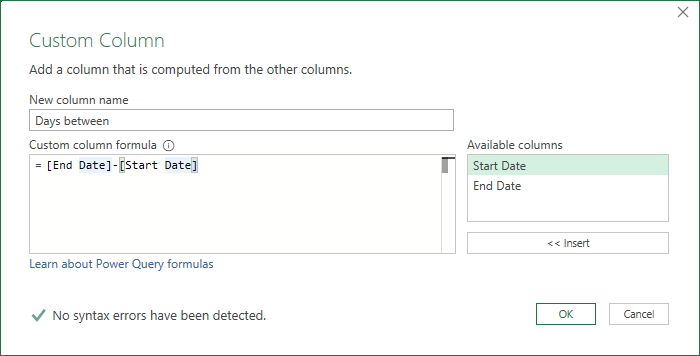
Click OK to accept the formula.
Finally, in Power Query, we change the data type of the new column to a whole number.
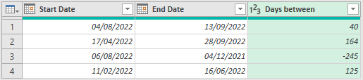
The result is a column with the number of days between the two dates.
The same +1 principle applies if we wish to include both the start and end dates. If so, the formula would be:
=[End Date]-[Start Date]+1Power Query Duration.Days function
Power Query does not have the same formulas as Excel. Instead, it has formulas written in a language called M. One example, is the Duration.Days function.
Syntax
=Duration.Days(duration)Arguments
- Duration – must be a valid duration data type or the difference between two dates
With the data loaded into Power Query, add a Custom Column and enter the following formula:
=Duration.Days([End Date]-[Start Date])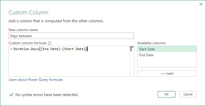
After clicking OK, change the data type to a whole number.
This provides the same result as the example above. The column displays the number of days between the two dates.
Remember, if you want to include both dates to +1 in the calculation.
=Duration.Days([End Date]-[Start Date])+1Conclusion
In this post, we have seen many different ways to calculate the number of days difference between two dates. Hopefully, in all these options, there is a solution that meets the needs of your scenario.
There is no built-in Power Query equivalent to NETWORKINGDAYS. This post contains a custom function which we can use instead: Working Days between Dates in Power Query – Gorilla.BI
Be careful when switching between solutions; The functions move the start and end date between the first argument and the second argument.
Discover how you can automate your work with our Excel courses and tools.
The Excel Academy

Make working late a thing of the past.
The Excel Academy is Excel training for professionals who want to save time.