Power Query – Unstacking data in a column

As we continue through this Power Query series, we have now reached a common and frustrating data format; data stacked in a column.  In this post, we will investigate one basic method for unstacking data.

While the example we are looking at below would most likely be created by a person who didn’t know how to structure data correctly, this format can equally be found in data exported, or copied from a IT system (though exported or copied data tends to be a single column, which is slightly easier to handle).

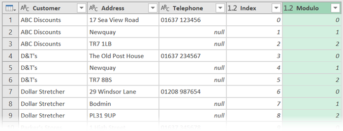
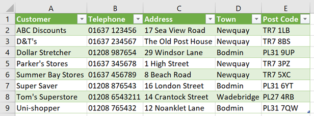
The screenshot below shows the Address has data stacked in a column.

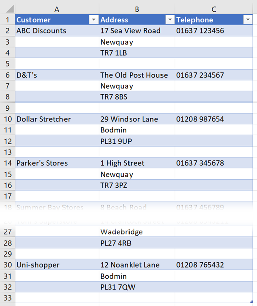
As you can imagine, manipulating data in this layout is exceptionally difficult.  To make it useable, each row of the address should be a separate column.  Power Query comes to the rescue once again.

Unstacking a column of data

Open the Example 1 worksheet from the downloaded file.  The data looks like the screenshot we saw above.

The data is already in a Table format, which I have named Customers.  To import the data into Power Query, select any cell in the Table and click Data -> From Table/Range from the ribbon.

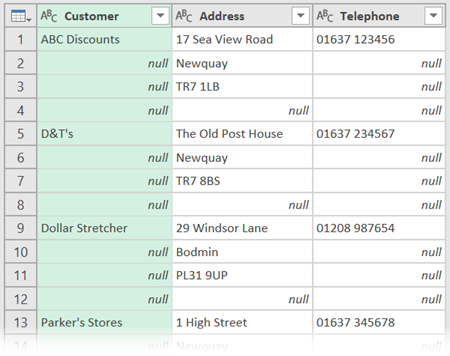
The Power Query window will open and display the data, which will look like the screen show below:

Tidy up the import

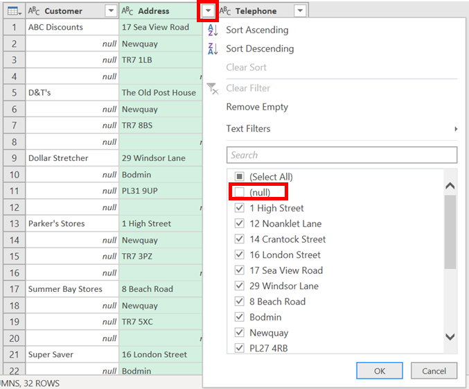
Now let’s work through the steps to get the separate address lines into columns.  First, let’s remove any blank rows by filtering the Address column to remove null values.

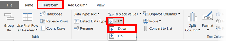
Click on the Customer column, then click Transform -> Fill (dropdown) -> Down from the ribbon.  This will ensure each row has the customer name in it; there should not be any null values in the Customer column.

Adding an Index and Modulo column

For the next few transformations, things start to seem a bit odd.  Once all the steps are complete, it will make sense, but until then you’ll just have to trust me.

There are 3 rows for every customer address.  Our next transformations are to include a column of numbers which show the numbers 0, 1 and 2 repeatedly.  0 will represent the first row of the address, 1 the second row of the address, and 2 the last line of the address.

Click Add Column -> Index Column

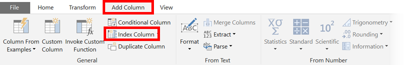
An index column has been added, starting at zero.

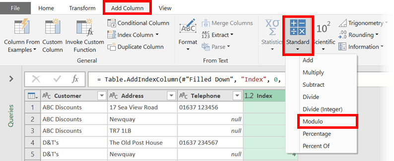
Select this new Index column, then click Add Column -> Standard -> Modulo.

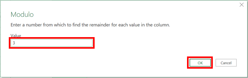
Enter 3 into the Modulo window, as there are 3 rows in each address.  Click OK.

If you’ve followed all the steps above the Preview Window should look like the screenshot below:

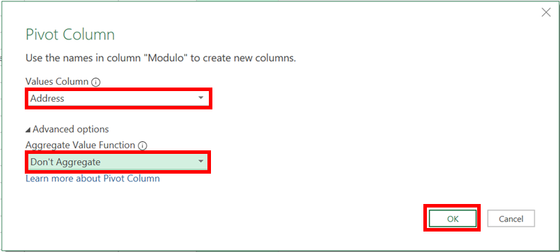
Select the Modulo column we created.  Click Transform -> Pivot Column.  In the Pivot Column window select the Address column, expand the advanced options, and select Don’t Aggregate, then click OK.

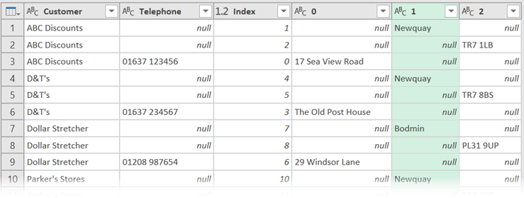
Take a look at the preview window, you probably think we’ve broken everything, but it’s all part of the process. We are about to bring this thing back into order.

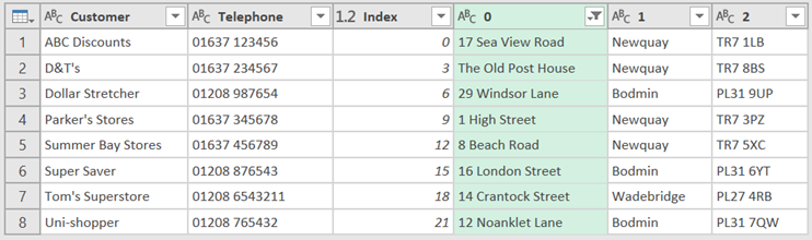
Select the columns with the headers 1 and 2, then apply the Transform -> Fill Down transformation.

Select the 0 column and filter to remove the null values.  The Preview Window will now show the data in the following format:

Magic eh? We went from thinking that everything was broken, to a nice and tidy data set in just a few basic transformations.

One of the critical skills for Power Query is the ability to make lots of small transformations which eventually add-up get the data into the right format.  Often something which may seem like a small transformation, such as unstacking data, may require a lot of smaller steps.

Finishing up

Just a few simple transformations remain to tidy everything up:

• Remove the Index column (Select the column and click Home -> Remove Columns)
• Rename the 0, 1 and 2 columns (double-click each column heading and provide a meaningful name).

That’s it.  The data is now ready.  Click Close and Load to push the data into Excel.

What does this teach us?

In this post, we’ve seen how to unstack a column of data.  But more importantly, we’ve seen that outcomes which might seem basic can be quite complex.  Understanding simple transformations and how to combine them together is something which takes time and thought to learn.

There are other methods for unstacking data, while they take less steps, they are more complex for a beginner to understand, so are beyond the scope of this beginners series.

---

What next?

Discover how you can automate your work with our Excel courses and tools.