How to use dynamic arrays with other features (7 scenarios)

So far, in this series, we’ve looked at how dynamic arrays work and the new functions that are available to us. Most of our examples have focused on calculations that occur on the worksheet. But we’ve not yet considered how dynamic arrays work with other Excel features, such as charts, data validation, conditional formatting, etc. So, we’re going to cover that in this post.

We won’t look at every Excel feature, but focus on the most common that we are likely to use dynamic arrays for.

Table of Contents

• Overview
• Arrays vs. ranges
• Tables
• Name manager
• Arrays
• Spill ranges (# references)
• Using named ranges with other features
• Charts
• Linked pictures
• PivotTables
• Conditional formatting
• Data validation
• Conclusion

Overview

When thinking about dynamic arrays, it’s useful to make a clear distinction between ranges and arrays. We often use these terms interchangeably, but they are not the same, and Excel certainly applies them differently. If we have a clear grasp of this, it will be easier to understand how dynamic arrays behave the way they do.

Arrays vs. ranges

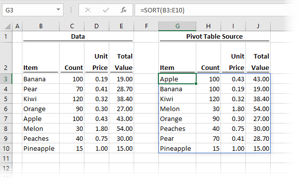
Excel converts data between arrays and ranges without the user even being aware. Let’s think about the journey our data goes through by using the SORT function as an example. We have some source data in cells B3-C5.

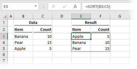
The formula in cell E3 is:

=SORT(B3:C5)

When we use the SORT function, what is actually happening:

1. The range B3:C5 is converted to an array: {“Banana”,10;”Pear”,15;”Apple”,5}
2. The SORT calculation is performed on the array, turning it into {“Apple,5;”Banana”,10;”Pear”,15}
3. The result of the array is returned into cell E3
4. Once the result exists on the worksheet, it becomes a range which we can refer to as E3#
5. Even though # references are on the face of the worksheet, when called, Excel still needs to recalculate to understand the size of the range as E3:F5.

This means that, generally speaking, the following statements hold true:

• Features that can handle arrays and perform calculations can contain dynamic array formulas
• Features that can handle calculations, but not arrays, can use the # referencing system
• Features that cannot perform calculations must use other methods to handle this for them.

Tables

Dynamic arrays have a love/hate relationship with Excel tables.

If we use Excel tables as the source for a dynamic array formula, everything works brilliantly. If new data is added to the table, the dynamic array formula updates automatically to include the new data. That’s the love part.

However, try to do the inverse and put a dynamic array formula inside an Excel table, and we get the #SPILL! error. That is the hate part. Arrays are about values, and tables hold values, so why is there a problem?

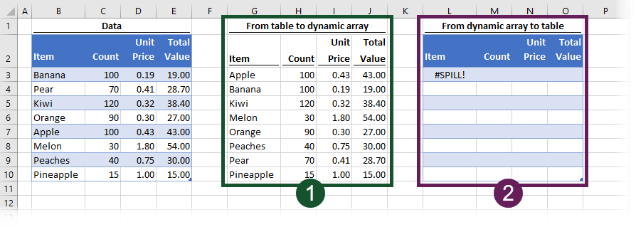
In the screenshot above:

1. Cell G3 contains the following formula:

   =SORT(Table1)

   This uses the full range of values from Table1 and outputs on the face of the worksheet.
2. The formula in cell L3 is:

   =G3#

   This cell reference is the spill range starting in cell G3, but it always results in a #SPILL! error.

Why does (1) work and (2) does not?

1. When using a dynamic array function with a table as its source, it is converting the table into an array and then returning that result somewhere else on the worksheet. It[‘s a simple calculation process.
2. When using a dynamic array inside a table, it causes issues. Both items are containers for auto-expanding data and perform automatic calculation. So, if you try to put something which auto-expands and auto-calculates into something else that also auto-expands and auto-calculates, what should happen? Which should expand first? Which should calculate first? What if one grows outside the bounds of the other? There are just too many questions without obvious answers. Since we have two competing features trying to achieve a similar outcome, the #SPILL! error is probably the best we can expect.

Name manager

A reader once commented to me that they thought named ranges were misnamed, that they should be called named formulas. I have come to agree, as the name manager can hold a host of other things such as constants, arrays, Excel 4 macros, and formulas.

In this section, we’ll look at just two items (1) arrays and (2) spill ranges.

Arrays

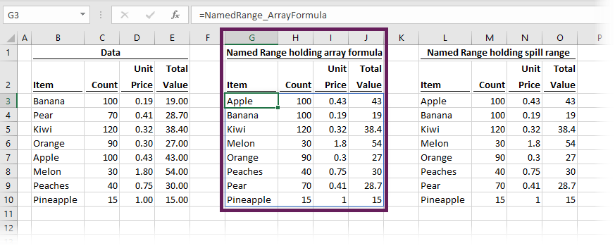
As the name manager can hold arrays and formulas, it is more than happy to hold dynamic array functions directly too. The screenshot below shows a named range containing the SORT function.

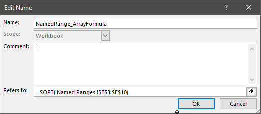
We can output the named range on the face of the worksheet (as shown in the screenshot below, cell G3 and its spill range), or use it in features that accept arrays.

Spill ranges (# references)

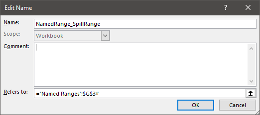
The name manager is also happy to hold # spill references, but we need to be careful about their creation. While named ranges can be used with absolute or relative cell references, to reference a spill range correctly, we must ensure the $ symbols are used to create an absolute reference.

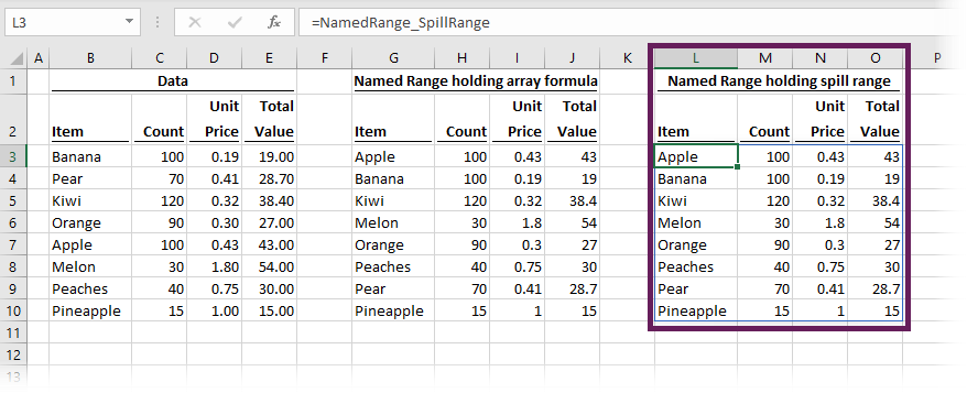
The named range created in the screenshot above has been used in the screenshot below (Cell L3 and its spill range)

Using named ranges with other features

As we go through the remainder of this post, you will see that named ranges are key to using dynamic arrays with many other features.

Even though a spill range is recognized as a range for formulas, it appears that Excel needs to perform some background processing to work out how big the range is. The name manager can perform calculations, so it can trigger this processing. Features that don’t contain any calculations can use named ranges as their source to handle the calculation element for them. We’ll look at this further in the sections below.

Charts

Charts can be a little picky about dynamic ranges already. I believe this is because the charting engine does not try to calculate any ranges, but just wants to use the range it has been given. This hasn’t changed with the introduction of dynamic arrays; it has always been the case. Even before dynamic arrays, if we wanted to use formulas such as INDEX or OFFSET to create a dynamic range, we needed to place it in a named range.

The screenshots below demonstrate that using a spill range directly in a chart source will result in an error.

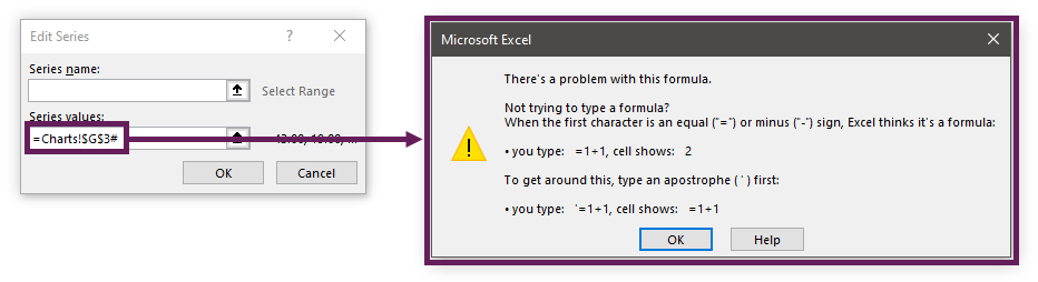
Instead, we need to use a named range containing a spill reference.

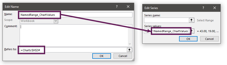
It should be noted that the output of the named ranges must be of the right type of data for the chart element. By which, I mean that named ranges used for chart values must contain numbers and named ranges used for axis labels must contain text values.

Update for Excel 365 users:

Excel 365 users have an additional feature that is not available in Excel 2021; the ability to tie a chart data range to an entire dynamic array range. For example, if a chart uses cells B3:E10 as the source, and that range is also the same as an existing spill range, Excel assumes the chart source is intended to be the same as the spill range. Therefore the chart range changes as the spill range changes.

Linked pictures

Linked pictures are similar to charts; they don’t try to calculate anything; they just want to display the range they are given. Therefore, using a # reference directly inside a linked picture doesn’t work. Therefore, we need to turn to the name manager once again.

The screenshot below shows a picture linked to a named range called NamedRange_LinkedPicture. That named range contains a dynamic array calculation.

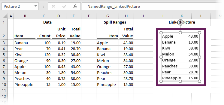
When the named range recalculates, the rows and columns may increase or decrease. The picture also then grows or shrinks to match the size of the named range.

For the purposes of demonstration of another technique, I’ve pulled a bit of Excel trickery in the named range used in the linked picture above. I have joined two spill ranges together into a single named range (as shown in the screenshot below).

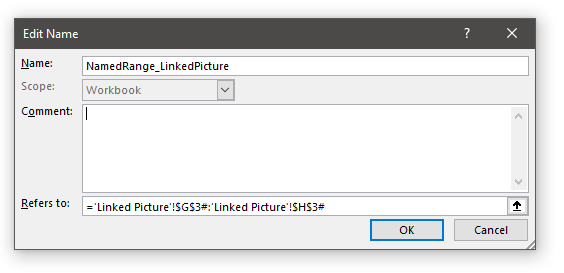
The formula in the name manager is:

='Linked Picture'!$G$3#:'Linked Picture'!$H$3#

These are two separate spill ranges, which have been combined as a single range using a colon in between. This creates a range that goes from G3 down to the end of the spill range for H3#.

PivotTables

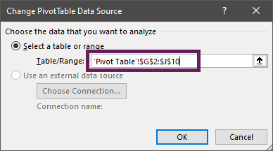
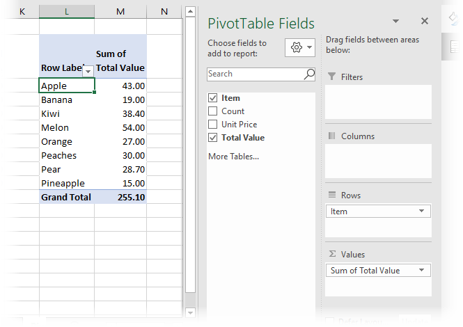
Initially, Pivot Tables appear to be happy using the # reference as a source, as shown by the screenshot below.

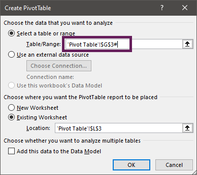
But don’t be fooled, as soon as we click OK, Excel converts the # reference to a standard static range and then creates the Pivot Table. The screenshot below shows that ‘Pivot Table’!$G$3# has been converted to a static range ‘Pivot Table’!$G$3:$J$10

Instead, we must turn to named ranges once again.

PivotTables make an assumption about our data, which is that the first row is the header row. This gives us an issue as # references often do not include the header. Instead, we can pull some more Excel trickery.

If our data is as follows:

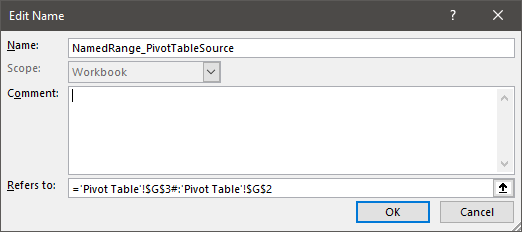
To include the header row, we can use the following formula in a named range; it creates a range from G2 to the bottom of the G3# spill range.

='Pivot Table'!$G$3#:'Pivot Table'!$G$2

Here is the formula used within a named range.

We can now use the named range as the source for the Pivot Table.

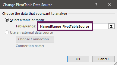
This now correctly includes the header row so that we can use it for the Pivot Table (as shown below).

Update for Excel 365 users:

In late 2022 new dynamic array formulas were released. One of those formulas is VSTACK, which enables us to stack dynamic arrays together into a single array. Therefore we no longer need to use range trickery to achieve the same result.

Conditional formatting

Conditional formatting is not compatible with dynamic arrays. If we use # references inside a conditional format, Excel converts it to a static range and it is no longer dynamic.

The screenshot below demonstrates that when using a spill range ($B$3#), clicking Apply converts the range to a static range ($B$3:$E$10).

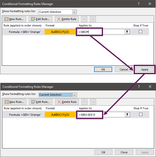
To use conditional formatting with dynamic arrays, we must select a static range that is bigger than our likely output. That will give the appearance of being dynamic, but may need maintenance from time to time when the spill range expands further than the conditionally formatted cells.

Data validation

Data validation lists perform calculations; but they only work with ranges; they cannot hold arrays. Therefore, a data validation list:

• Can use the # referencing system.
• Can use a named range which uses a range (including the # referencing system).
• Cannot hold a dynamic array formula or use a named range that outputs an array.

The screenshot below shows a data validation list containing the spill range starting in cell G3. The # referencing system is based on a range, therefore it will operate correctly in this scenario.

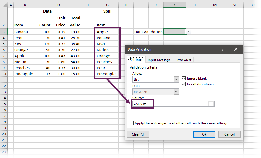
Note: The data must be in the right shape to work with data valuation, so it must be a single row or column.

Conclusion

We’ve seen that many Excel features are directly compatible with dynamic arrays. And for most features that aren’t, we can use the name manager to bridge the gap. By looking at the general rules, it has provides a good understanding of how dynamic arrays operate when used with other Excel features.

Want to learn more?

There is a lot to learn about dynamic arrays and the new functions. Check out my other posts here to learn more:

• Introduction to dynamic arrays – learn how the excel calculation engine has changed.
• UNIQUE – to list the unique values in a range
• SORT – to sort the values in a range
• SORTBY – to sort values based on the order of other values
• FILTER – to return only the values which meet specific criteria
• SEQUENCE – to return a sequence of numbers
• RANDARRAY – to return an array of random numbers
• Using dynamic arrays with other Excel features – learn to use dynamic arrays with charts, PivotTables, pictures etc.
• Advanced dynamic array formula techniques – learn the advanced techniques for managing dynamic arrays

---

What next?

Discover how you can automate your work with our Excel courses and tools.