RANDARRAY function in Excel (How to + 4 Examples)

The RANDARRAY function makes use of the changes made to Excel’s calculation engine. These changes enable a single formula to spill results into multiple cells. The regular RAND function calculates a single random number, which is greater than or equal to zero and less than 1. The RANDARRAY function calculates a random number in the same way, but the user can specify the number of rows, columns, minimum, maximum and rounding of the random numbers returned.

At the time of writing, the RANDARRAY function is only available in Excel 2021, Excel 365, and Excel Online. It will not be available in Excel 2019 or earlier versions.

Table of Contents

• Arguments of the RANDARRAY function
• Examples of using the RANDARRAY function
• Example 1 – Basic usage
• Example 2 – Using RANDARRAY with SORTBY
• Example 3 – Using all the arguments of RANDARRAY
• Example 4 – Replacing RAND and RANDBETWEEN

Watch the video:

Watch the video on YouTube

Arguments of the RANDARRAY function

RANDARRAY has five arguments, all of which are optional.

=RANDARRAY([Rows], [Columns], [Min], [Max], [Integer])

• [Rows]: The number of rows of random numbers to return. If this argument is excluded, the default is 1.
• [Columns]: The number of columns of random numbers to return. If this argument is excluded, the default is 1.
• [Min]: The lowest number to be returned. If excluded, the default is 0.
• [Max]: The highest value to be returned. If excluded, the default value is 0.999999999999999 (i.e., just less than 1)
• [Integer]: Can be set as:
  • TRUE = return whole numbers only
  • FALSE = return decimal values to 15 decimal places
  If excluded, the default is FALSE.

As all the arguments are optional, we can use RANDARRAY() without any arguments to create a single random number.

One attribute to be aware of is that RANDARRAY is a volatile function. This means that it recalculates every time any cell changes. If you’ve used the RAND function before, this functionality will not be new to you.

Examples of using the RANDARRAY function

The following examples illustrate how to use the RANDARRAY function.

Example 1 – Basic usage

In the screenshots below, we see basic examples of using the RANDARRAY function.

Single dimension

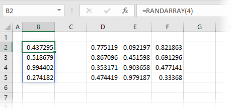
The formula in cell B2 is:

=RANDARRAY(4)

The formula above creates an array of random numbers which is four rows and one column in size.

Multiple dimensions

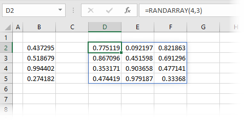
The formula in cell D2 is:

=RANDARRAY(4,3)

The formula above creates an array of random numbers which is four rows and three columns in size.

Example 2 – Using RANDARRAY with SORTBY

This example shows how to turn a sorted list into a random order.

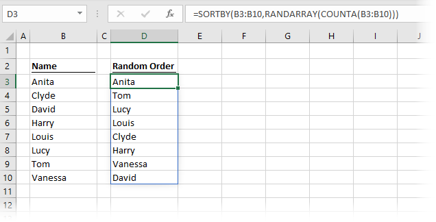
The formula in cell D3 is:

=SORTBY(B3:B10,RANDARRAY(COUNTA(B3:B10)))

RANDARRAY(COUNTA(B3:B10)) creates a list of random numbers which is the same size as the source data. SORTBY is then used to put cells B3-B10 into the order of the random numbers.

Example 3 – Using all the arguments of RANDARRAY

In the screenshot below, we can see all the arguments of the RANDARRAY function in Excel.

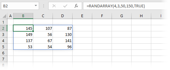
The formula in cell B2 is:

=RANDARRAY(4,3,50,150,TRUE)

The formula creates an array of results which is four rows, three columns, a minimum of 50, a maximum of 150, with only whole numbers.

Example 4 – Replacing RAND and RANDBETWEEN

There are two existing functions in Excel that already create random numbers: RAND and RANDBETWEEN. We no longer need these functions, as RANDARRAY can replace both of these.

Replacing RAND

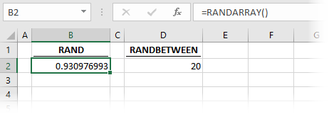
The formula in cell B2 is:

=RANDARRAY()

The default options applied by the RANDARRAY function provide the same result as the RAND function.

Replacing RANDBETWEEN

The RANDBETWEEN function selects integers between an upper and lower limit.

The formula in cell D2 is:

=RANDARRAY(,,10,20,TRUE)

This demonstrates that RANDARRAY has the ability to select a minimum, maximum and return integers. Therefore, RANDARRY provides the same result as RANDBETWEEN.

Want to learn more?

There is a lot to learn about dynamic arrays and the new functions. Check out my other posts here to learn more:

• Introduction to dynamic arrays – learn how the excel calculation engine has changed.
• UNIQUE – to list the unique values in a range
• SORT – to sort the values in a range
• SORTBY – to sort values based on the order of other values
• FILTER – to return only the values which meet specific criteria
• SEQUENCE – to return a sequence of numbers
• RANDARRAY – to return an array of random numbers
• Using dynamic arrays with other Excel features – learn to use dynamic arrays with charts, PivotTables, pictures etc.
• Advanced dynamic array formula techniques – learn the advanced techniques for managing dynamic arrays

---

What next?

Discover how you can automate your work with our Excel courses and tools.