SORTBY function in Excel (How to + 6 Examples)

The SORTBY function was announced by Microsoft in September 2018 and is one of Excel’s new dynamic array functions. SORTBY makes use of the changes made to the calculation engine, enabling a single formula to spill calculations into multiple cells.

At the time of writing, the SORTBY function is only available in Excel 365, Excel 2021 and Excel Online. It will not be available in Excel 2019 or earlier versions.

Table of Contents

• Arguments of the SORTBY function
• Examples of using the SORTBY function
• Example 1 – The sort column does not need to be in the array
• Example 2 – SORTBY expands automatically when linked to a table
• Example 3 – Using SORTBY with multiple columns
• Example 4 – Returning columns in any order when using SORTBY
• Example 5 – Combining FILTER and SORTBY
• Example 6 – Restrict the values returned by SORTBY

Watch the video:

Watch the video on YouTube

Arguments of the SORTBY function

Before we look at the arguments required for the SORTBY function, let’s look at a basic example to appreciate what it does.

The video below is sorting the Employees based on the Units Sold; this is what SORTBY does. The returned range returned does not need to include the values that it is being sorted by. That’s pretty useful, right?

SORTBY has a variable number of arguments depending on the scenario:

=SORTBY(array, By_array1, [sort_order1], [By_array2], [sort_order2] ,...)

• array: The range of cells, or array of values to be returned by the function.
• by_array1: The range of cells or array of values to sort by.
• [sort_order1]: acceptable values are:
  • 1 = sort By_array1 in ascending order
  • -1 = sort By_array1 in descending order
  If excluded, Excel defaults to 1.
• [by_array2…]: The range of cells or array of values to apply the second sort by. This argument is optional; you can exclude this if you only need one sort column.
• [sort_order2]: the sort order to apply to the By_array2. Uses the same values as sort_order1, where 1= ascending, -1 = descending.

If there is a third, fourth or nth sort required, these can be added just like by_array2 and sort_order2.

Only the first two arguments are necessary, which are the data and what to sort by. If you don’t need to sort by a separate column, then the SORT function may be better suited to your requirements.

Examples of using the SORTBY function

The following examples illustrate how to use the SORTBY function in Excel

Example 1 – The sort column does not need to be in the array

In this example, the Employees, Units Sold and Average Price columns are returned based on the descending order of the values in the Total Value column.

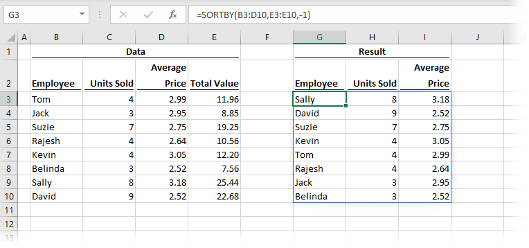
The formula in cell G3 is:

=SORTBY(B3:D10,E3:E10,-1)

Cells B3-D10 are sorted by the values in E3-E10 in descending order (it is descending because the third argument in the function is -1). The Total Value column (cells E3-E10) is not included within the result.

Example 2 – SORTBY expands automatically when linked to a table

This example shows how the SORTBY function responds when new data is added to an Excel Table.

The SORTBY function is using a table called salesTable as its source. New records added to the Table are automatically added to the spill range of the function. There is no need to expand the range of the function; it happens all by itself.

Example 3 – Using SORTBY with multiple columns

Example 3 shows how to sort using multiple sort columns.

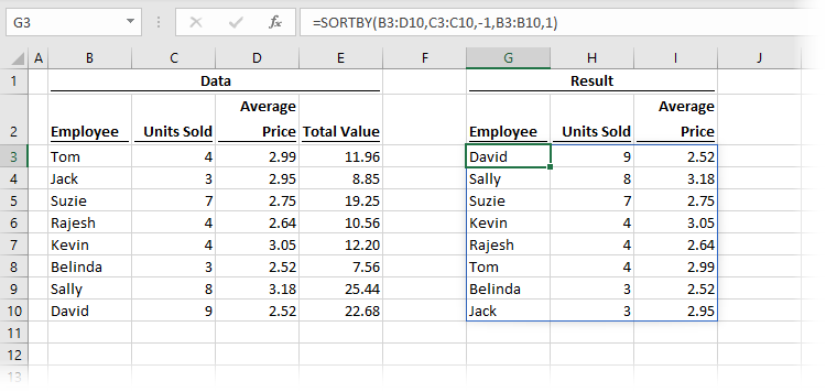
The formula in cell G3 is:

=SORTBY(B3:D10,C3:C10,-1,B3:B10,1)

Cells B3-D10 are sorted first by cells C3-C10 (the Units Sold) in descending order, then by cells B3-B10 (the Employee name) in ascending order.

Example 4 – Returning columns in any order when using SORTBY

SORTBY accepts a range or array as the first argument. It then returns the columns in the result in the same order. But what if we want a different order, or only wish to return a few of the columns? In this circumstance, we can use the CHOOSE function to create a range of cells in any order. This solution will working in Excel 2021 and Excel 365.

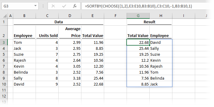
The formula in cell G3 is:

=SORTBY(CHOOSE({1,2},E3:E10,B3:B10),C3:C10,-1,B3:B10,1)

The CHOOSE function is using E3-E10 as the first range, and B3-B10 as the second range. The {1,2} is telling the CHOOSE function which position each range should be in. If you were to use {2,1}, the ranges would be returned in the reverse order.

Using this method, we can return columns in any order; we are not restricted by the layout of the source data.

For Excel 365 users there is the CHOOSECOLS function available which makes this scenario even easier. The following are two examples of using CHOOSECOLS to achieve the same result.

=CHOOSECOLS(SORTBY(B3:E10,C3:C10,-1),4,1)

=CHOOSECOLS(SORTBY(B3:E10,C3:C10,-1),{4,1})

Example 5 – Combining FILTER and SORTBY

The dynamic array functions can be nested within each other. But this nesting can bring some challenges. This example shows the FILTER function nested within SORTBY.

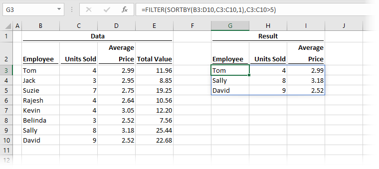
The formula in cell G3 is:

=FILTER(SORTBY(B3:D10,C3:C10,1),C3:C10>5)

This formula is intended to sort based on cells C3-C10, then filter to only return the rows where the values in C3-C10 are greater than 5.

But did you notice in the screenshot that it doesn’t return the correct values? This occurs because the first argument of the FILTER function uses SORTBY to sort, but the second argument is using the unsorted data. When nesting these formulas, we need to apply the sort to each argument.

Let’s try it again…

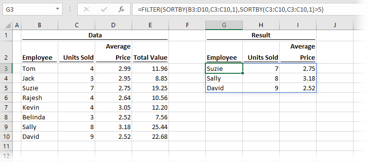
The formula in cell G3 is:

=FILTER(SORTBY(B3:D10,C3:C10,1),SORTBY(C3:C10,C3:C10,1)>5)

Now both arguments of the FILTER function are based on arrays sorted by C3-C10.

Example 6 – Restrict the values returned by SORTBY

Finally, what if you only want to return a single sort position? For example, what if we only wanted the 3rd item from the sorted list?

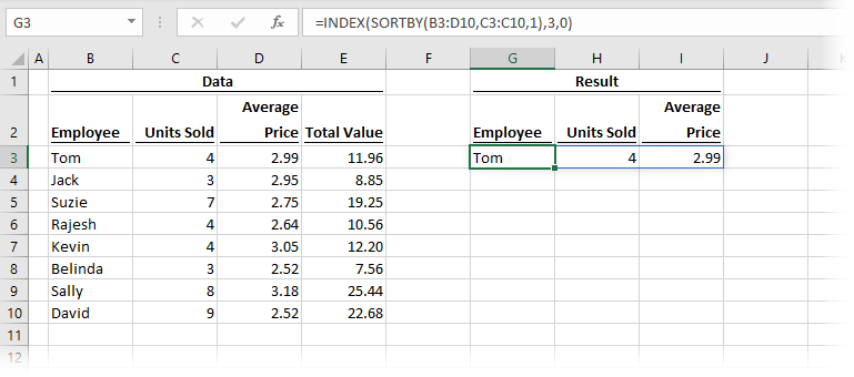
The formula in cell G3 is:

=INDEX(SORTBY(B3:D10,C3:C10,1),3,0)

SORTBY is nested within the INDEX function. It is the INDEX function that is returning the 3rd item in the list. This solution works in Excel 2021 and Excel 365.

An alternative option using CHOOSEROWS (only available in Excel 365) is:

=CHOOSEROWS(SORTBY(B3:D10,C3:C10,1),3)

Want to learn more?

There is a lot to learn about dynamic arrays and the new functions. Check out my other posts here to learn more:

• Introduction to dynamic arrays – learn how the excel calculation engine has changed.
• UNIQUE – to list the unique values in a range
• SORT – to sort the values in a range
• SORTBY – to sort values based on the order of other values
• FILTER – to return only the values which meet specific criteria
• SEQUENCE – to return a sequence of numbers
• RANDARRAY – to return an array of random numbers
• Using dynamic arrays with other Excel features – learn to use dynamic arrays with charts, PivotTables, pictures etc.
• Advanced dynamic array formula techniques – learn the advanced techniques for managing dynamic arrays

---

What next?

Discover how you can automate your work with our Excel courses and tools.