SORT function in Excel (How to + 6 Examples)

The SORT function in Excel, is one of Excel’s best new features. It’s one of a group of functions that make use of Excel’s new dynamic array calculation engine, enabling Excel to spill results into multiple cells from a single formula.

At the time of writing, the SORT function is only available for Microsoft 365, Excel 2021 and Excel Online. It will not be available in Excel 2019 or earlier versions.

Download the example file: Click the link below to download the example file used for this post:

Watch the video:

Watch the video on YouTube

Arguments of the SORT function in Excel

Before we look at the arguments required for the SORT function, let’s look at a basic example to appreciate what it does.

As demonstrated below, the SORT function does exactly what you would expect; it sorts the data. The critical point is to notice that it achieves this with a single function in a single cell and spills the other results into the cells below.

SORT has four arguments:

=SORT(array, [sort_index], [sort_order], [by_col])

• array: The range of cells, or array of values to be sorted.
• [sort_index]: The nth column or row to apply the sort to. For example, to sort by the 2nd column, the sort index would be 2. It is possible to sort by multiple columns (covered in Example 6 below). If this argument is excluded, Excel defaults to sorting by the first column.
• [sort_order]: contains either:
  • 1 = sort in ascending order
  • -1 = sort in descending order
  If excluded the argument defaults to 1.
• [by_col]: can be either:
  • TRUE = sort by columns
  • FALSE = sort by rows
  If excluded the argument defaults to FALSE.

Examples of using the SORT function

The following examples illustrate how to use the SORT function.

Example 1 – SORT returns an array of rows and columns

In this example, a single formula sorts the values in the first column and returns the full range of cells provided by the array argument.

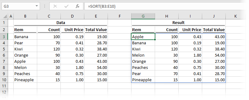
The formula in cell G3 is:

=SORT(B3:E10)

This single formula is returning eight rows and four columns of data. As the second, third, and fourth arguments have been excluded, the defaults are applied for each of them, sorting by the first column, in ascending order with data organized in rows.

Example 2 – SORT by another column in descending order

Example 2 shows how to sort by the second column in descending order.

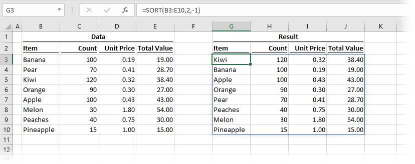
The formula in cell G3 is:

=SORT(B3:E10,2,-1)

The second argument in the SORT function is the sort_index. Therefore, by using 2 as the sort_index, the formula above is sorted by the 2nd column of the array.

The third argument is the sort_order. The -1 in this argument denotes the data sorts in descending order.

Example 3 – SORT expands automatically when linked to a Table

The animation below shows how the SORT function responds when linked to an Excel table.

In this example, the SORT function is using an Excel Table as its source data array. New records added to the Table are automatically added to the spill range of the function.

Example 4 – Using SORT to return a top 5 and specific columns

Example 4 shows how to create a top 5 and select which specific columns to return. As this example also uses the INDEX and SEQUENCE functions, it will work in Excel 2021 and Excel 365.

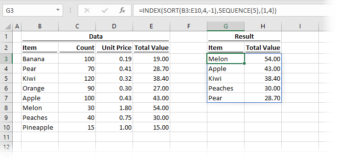
The formula in cell G3 is:

=INDEX(SORT(B3:E10,4,-1),SEQUENCE(5),{1,4})

We are using two additional functions in this example, SEQUENCE (also a new function) and INDEX (which is not new, it has been around forever).

SORT is applied to the 4th column in descending order, we have seen similar examples to this above.

INDEX takes the result of the SORT function and uses:

• The SEQUENCE function to only show the first 5 results
• A constant array to display only columns 1 and 4.

In the past, this would have needed a lot of calculations, but now it’s possible with a single function – Amazing!

If using Excel 365, an alternative function that uses the CHOOSEROWS and CHOOSECOLS can be found below:

=CHOOSECOLS(CHOOSEROWS(SORT(B3:E10,4,-1),SEQUENCE(5)),1,4)

=CHOOSECOLS(CHOOSEROWS(SORT(B3:E10,4,-1),SEQUENCE(5)),{1,4})

In both of these, SEQUENCE creates an array {1,2,3,4,5}, which is used inside the CHOOSEROWS function to return only the first 5 rows. CHOOSECOLS then returns only columns 1 and 4.

Example 5 – Combining FILTER and SORT

The dynamic array functions can be nested within each other. This example shows the FILTER function nested inside SORT.

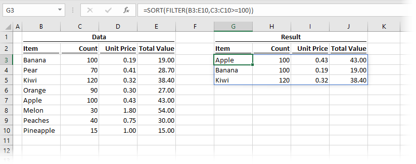
The formula in cell G3 is:

=SORT(FILTER(B3:E10,C3:C10>=100))

The FILTER function returns only three rows, where the values in cells C3-C10 are 100 or higher. SORT is then applied to the result of the FILTER, to provide those filtered rows in alphabetical order.

Example 6 – SORT on multiple columns

SORT can be applied to multiple columns at the same time.

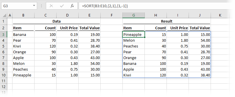
The formula in cell G3 is:

=SORT(B3:E10,{2,1},{1,-1})

This formula contains two constant arrays. The first, {2,1} is the sort_order, which in this example is sorting by column 2 then by column 1. The second constant array is {1,-1}, which determines how each column sorts. The first sort (applied to column 2) is in ascending order, and the second sort (applied to column 1) is in descending order.

Want to learn more?

There is a lot to learn about dynamic arrays and the new functions. Check out my other posts here to learn more:

• Introduction to dynamic arrays – learn how the excel calculation engine has changed.
• UNIQUE – to list the unique values in a range
• SORT – to sort the values in a range
• SORTBY – to sort values based on the order of other values
• FILTER – to return only the values which meet specific criteria
• SEQUENCE – to return a sequence of numbers
• RANDARRAY – to return an array of random numbers
• Using dynamic arrays with other Excel features – learn to use dynamic arrays with charts, PivotTables, pictures etc.
• Advanced dynamic array formula techniques – learn the advanced techniques for managing dynamic arrays