Advanced dynamic array formula techniques (3 methods)

In the final part of this series, we look at a few advanced dynamic array formula techniques. We won’t be covering the individual functions in detail but considering how we can combine them to solve some tricky problems. Many of these techniques have been covered briefly as examples in previous posts, but now we’ll dig deeper.

NOTE: In September 2022, Excel 365 users gained access to 14 new dynamic array functions (TEXTBEFORE, TEXTAFTER, TEXTSPLIT, VSTACK, HSTACK, TOROW, TOCOL, WRAPROWS, WRAPCOLS, TAKE, DROP, CHOOSEROWS, CHOOSECOLS, EXPAND). These functions provide easier methods and supersede many of the techniques discussed on this page. Therefore, Excel 365 users should explore these functions first. https://techcommunity.microsoft.com/t5/excel-blog/announcing-new-text-and-array-functions/ba-p/3186066

As Excel 2021 users do not currently have access to these functions, this page provides the best current information.

There are three key areas we’ll be covering:

• Single formula or cascading formula methodologies
• Useful supporting functions
• Using # References with the union operator

These are all separate topics, but when the techniques are combined, we can achieve some amazing things.

Table of Contents

• Single formula Vs. cascading formula methodology
• Cascading formulas
• Single formula
• Useful supporting functions
• CHOOSE
• INDEX
• SEQUENCE
• Using # references with union operator
• Conclusion

Single formula Vs. cascading formula methodology

When we write dynamic array formulas, we have some choices. One of which is whether to write multiple cascading or single aggregated formulas. There are advantages and disadvantages to each. Let’s look at an example to understand what we’re talking about.

Here is the data we’ll be using.

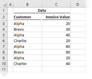
The goal of this example is to calculate the total invoice value for each customer using the UNIQUE and SUMIFS functions.

Cascading formulas

This first option uses two separate formulas in cells E3 and F3.

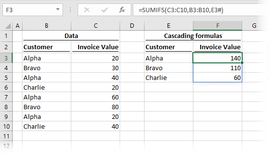
The formula in cell E3 is:

=UNIQUE(B3:B10)

This formula creates a distinct list of customers, and outputs the result into the spill range starting at cell E3. We’ve seen UNIQUE do this before in a previous post.

The formula in cell F3 is:

=SUMIFS(C3:C10,B3:B10,E3#)

This is a standard SUMIFS function using the spill range of the UNIQUE function in the last argument.

The point to note here is that there are two separate formulas to achieve the final result. The second formula relies on the spill range of the first to create its output.

Single formula

In this second scenario, we see that the same result can be created from a single formula.

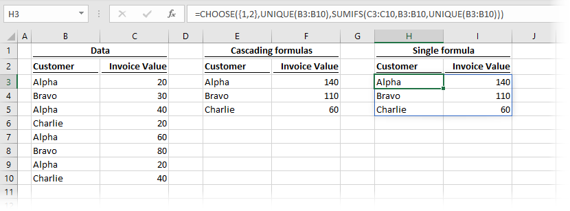
The formula in cell H3 is:

=CHOOSE({1,2},UNIQUE(B3:B10),SUMIFS(C3:C10,B3:B10,UNIQUE(B3:B10)))

We have used CHOOSE to combine the functions into a single array. The first column is the result of the UNIQUE and the second column is the result of the SUMIFS. As the spill range of the UNIQUE function does not exist on the face of the worksheet, we can’t use a # reference; instead, we repeat the UNIQUE function as the last argument of the SUMIFS.

Useful supporting functions

When working with dynamic arrays, there are many functions that help us to work with arrays. Three of the most useful are CHOOSE, INDEX, and SEQUENCE. We’ll consider each of these in this section.

CHOOSE

Having just looked at an example using CHOOSE, this seems like the obvious place to start.

CHOOSE can be used for array aggregation. In the example above, we took two separate arrays and combined them into one. As we have seen, this is useful for creating a single spill range by purposefully selecting the data to return.

INDEX

INDEX is a function that can be used to reduce the output of our array function.

Look at the example below.

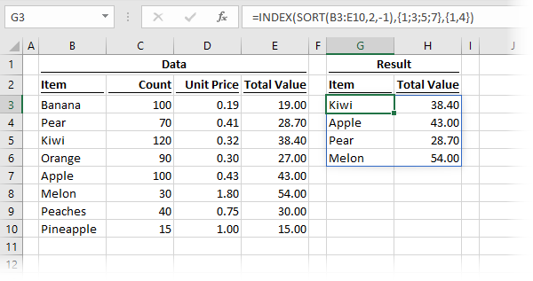
The formula in cell G3 is:

=INDEX(SORT(B3:E10,2,-1),{1;3;5;7},{1,4})

The SORT function is applied to cells B3-E10, in descending order based on column 2. For more examples of using SORT, check out this post.

The purpose of this example is not to demonstrate SORT, but to show how the INDEX function operates. In our scenario, INDEX is returning rows 1, 3, 5, and 7 and columns 1 and 4 from the array. Take note that when working with rows, the constant array is separated by semi-colons. But when used with columns, constant arrays are separated by commas.

INDEX Vs. CHOOSE – what’s the difference?

From the examples above, INDEX and CHOOSE appear to be performing similar tasks, but if you think about it, they are actually performing the opposite to each other. In this context, CHOOSE aggregates columns into a single array, while INDEX tasks a single array and selects the data to retain.

Using CHOOSE to aggregate data requires us to be explicit about what we combine. INDEX, however can be made more dynamic by using the SEQUENCE function to select which data to retain.

SEQUENCE

While SEQUENCE is a dynamic array function in its own right, it is also a great support function. In the example above, we used the INDEX function with fixed-size constant arrays. To build more dynamic functions, we can turn to the SEQUENCE function.

Look at the example below.

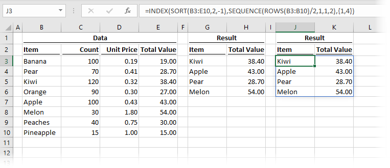
The result is the same as the previous example, but the formula in cell J3 is:

=INDEX(SORT(B3:E10,2,-1),SEQUENCE(ROWS(B3:B10)/2,1,1,2),{1,4})

SEQUENCE creates an array of alternate numbers, replacing the constant array used previously. By using SEQUENCE, each of the arguments can be linked to a cell, which means we could easily make this select every 3rd, 4th or nth row simply by changing a single cell value.

Using # references with union operator

As a final technique, let’s consider # spill references with the union operator. In this example, we will see how we can add additional data into a spill range by using a colon (which is the union operator) between cell addresses.

Let’s suggest we have a spill range starting at cell A2, and we want to include a header row into that spill range. We could use the following formula:

=A2#:A1

Excel understands this to be a range covering all the cells from A1 to the end of the spill range starting in A2. It does not matter how big the A2 spill range is; it will automatically expand or retract as necessary.

To illustrate this further, I would like to cover a technique discovered by Jon Acampora in this post: https://www.excelcampus.com/functions/total-rows-dynamic-arrays

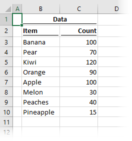
Here is the data we will be working with:

In this example, we want to return the items with a count greater than 100, but also include a header and total row.

First, let’s use the FILTER function to return only those items with a count greater than 100. This is nothing tricky; we’ve seen a lot of similar examples in the FILTER part of this series.

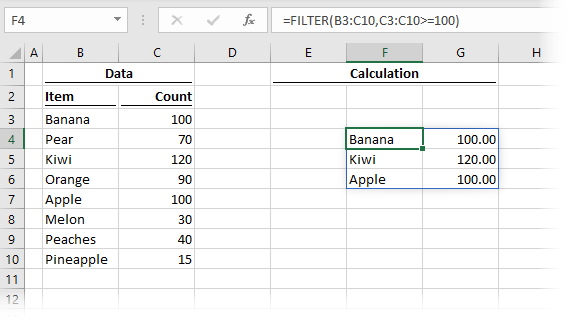
The formula in cell F4 is:

=FILTER(B3:C10,C3:C10>=100)

Next, let’s add column headers above the data. In cell F3, I’ve entered Item, and in G3, I’ve entered Count.

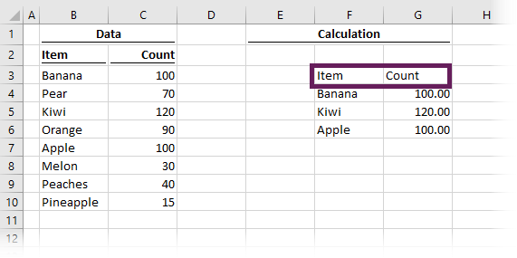
Now let’s add a total row.

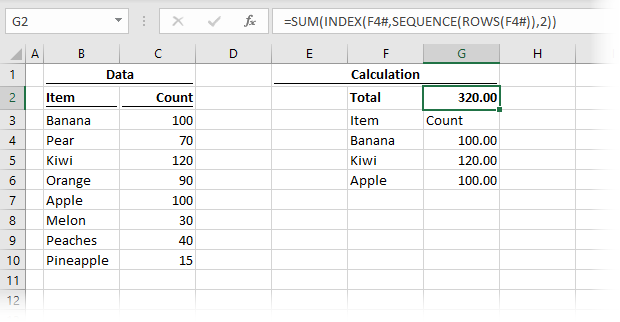
In cell F2, I’ve entered Total, and in cell G2, I’ve added the following formula:

=SUM(INDEX(F4#,SEQUENCE(ROWS(F4#)),2))

Hopefully, you’ll notice that we are applying the techniques from the sections above. In simple terms, this is returning the SUM of all the rows from the 2nd column of the spill range starting in F4.

The next step is to create an index number, which represents the order we wish to display the rows.

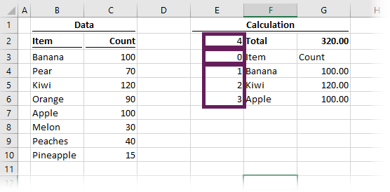
• The formula in cell E4 is:

  =SEQUENCE(ROWS(F4#)) 

• As the header row should come first, cell E3 has been given a hardcoded index of 0.
• Then the formula in cell E2 is calculating the number of rows in the spill range plus 1.

  =ROWS(E4#)+1

All we have to do now is use SORTBY to create a new spill range with the data displayed in the same order as the index column.

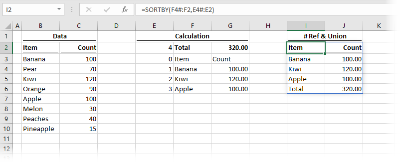
The formula in cell I2 is:

=SORTBY(F4#:F2,E4#:E2)

The key point to notice here are the two ranges:

• F4#:F2 is refers to a range that starts at cell F2 and finishes at the end of F4’s spill range.
• E4#:E2 is the range of index values we created

The biggest issue with this technique is that the final result is not automatically formatted.

• The header row won’t move, so we can format that using the standard tools.
• The total row can move depending on how our data changes (i.e., if the count of Melons increases to 150, the total row will have to move down to accommodate the additional data row). To format the total, we need to use conditional formatting with a big enough range to cover any potential growth.

Conclusion

Cascading spill ranges, support functions, and the union operator are all dynamic array formula techniques that we can use to make dynamic arrays even more flexible.

As you can see, the final example in this post incorporates a lot of our other formula techniques. It is worth taking the time to understand how it works; if you master this, then you’ll be able to achieve almost anything with dynamic arrays.

This is just the start; as more users get hold of the dynamic array functions, you can be sure that more formula techniques will be discovered. Maybe after reading this post, and understanding the concepts, you might discover the new techniques 👍

Want to learn more?

There is a lot to learn about dynamic arrays and the new functions. Check out my other posts here to learn more:

• Introduction to dynamic arrays – learn how the excel calculation engine has changed.
• UNIQUE – to list the unique values in a range
• SORT – to sort the values in a range
• SORTBY – to sort values based on the order of other values
• FILTER – to return only the values which meet specific criteria
• SEQUENCE – to return a sequence of numbers
• RANDARRAY – to return an array of random numbers
• Using dynamic arrays with other Excel features – learn to use dynamic arrays with charts, PivotTables, pictures etc.
• Advanced dynamic array formula techniques – learn the advanced techniques for managing dynamic arrays

---

What next?

Discover how you can automate your work with our Excel courses and tools.