Excel has changed… like seriously, changed. Every time we used Excel in the past, we accepted a simple operating rule; one formula one cell. Even with advanced formulas, it was still necessary to have a cell for each. But this has changed; Excel now allows a single formula to fill multiple cells. This is possible because Microsoft has changed Excel’s calculation engine to allow dynamic arrays.
The term dynamic arrays sounds complicated, but once you understand it, you’ll appreciate its simplicity and power.
Note: At the time of writing, dynamic arrays are available in Excel 365, Excel Online and Excel 2021 only. Excel 2019 and prior will not be updated to include dynamic arrays.
Table of Contents
Watch the video:

Overview of dynamic arrays
Let’s begin by looking at a basic example. Here is the formula:
=B2:B6OK, it’s not a formula you’ve ever used, but it’s simple enough to help describe the impact of dynamic arrays.
Before dynamic arrays
In Excel 2019 and prior, only one cell result could be returned by a formula. If we provided a formula with five results (cell B2, B3, B4, B5, and B6, as per our example), then some assumptions needed to be made by Excel. As a result, there are multiple outcomes from the formula above:
- If the formula was in line with the source data Excel assumed we want the value from the same row.
- If the formula was not in line with the source data, Excel got confused and returned the #VALUE! error.
Take a look at the screenshot below:
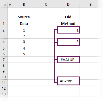
The value of 1 is shown in cell D2, as Excel assumes we want the value from cell B2 because it is in line with it. Had we entered exactly that same formula in cell D4, Excel assumes we want the inline cell, so returns 3 from cell B4.
Since cell D7 is not in line with any of the source data, Excel doesn’t know what we want, and returns the #VALUE! error. This assumption has got a technical name, implicit intersection. But we don’t really need to worry about that anymore.
It’s interesting to think that Excel could calculate different results from the same formula (hopefully a thing of the past). To override implicit intersection, Excel allowed us to press Ctrl+Shift+Enter when entering formulas. But we don’t need to worry about that anymore either.
With dynamic arrays
If we have a newer, dynamic array enabled version of Excel, there is only one possible result for our example formula; Excel returns all 5 cells. In the screenshot below, cell D2 contains the formula, but the result is shown in cells D2, D3, D4, D5 and D6. One formula displays 5 results… amazing!
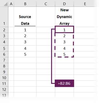
The basic rule of one formula one cell has gone. The terminology to describe a formula filling multiple cells is spilling, and the range of cells filled by that formula is called the spill range.
Which versions of Excel have dynamic arrays?
Microsoft originally announced the change to Excel’s calculation engine in September 2018. For over a year, it was only available to those who signed up to test early releases of the new features. Regular subscribers on the Microsoft 365 monthly update channel started to receive the update from November 2019. Finally, in July 2020, those on the semi-annual channel of the Microsoft 365 subscription (mostly business users) also received dynamic arrays.
Microsoft has already confirmed this new functionality will not be available in Excel 2019 or prior versions. So, if you want it, then it’s time to upgrade to Excel 2021 or a Microsoft 365 license.
New dynamic array functions
When Microsoft announced the new dynamic array functionality, they also introduced 6 new functions. All of which make use of this new calculation engine:
- UNIQUE – to list the unique or distinct values in a range
- SORT – to sort the values in a range
- SORTBY – to sort values based on the order of other values
- FILTER – to return only the values which meet specific criteria
- SEQUENCE – to return a sequence of numbers
- RANDARRAY – to return an array of random numbers
While we all get excited by new functions, the introduction of dynamic arrays is bigger than this; it’s a fundamental shift in how Excel (and Excel users) think about ALL formulas. In the remainder of this post, you get to understand the basics needed to start thinking in this new way.
Dynamic array formulas
As noted above, there are new functions that make use of this new spilling functionality. We won’t go into detail about each of these in this post; there are separate posts for each of them. The critical thing to realize is that the ability to spill is not restricted to these new functions; many existing functions now spill too.
Look at the example data below.
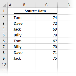
This is a simple scenario in which we have data in cells B2-C9. This data displays a name and a score. Let’s assume the goal is to calculate the total score for each person.
Before dynamic arrays
To calculate the total score for each individual, we could use the SUMIFS function.
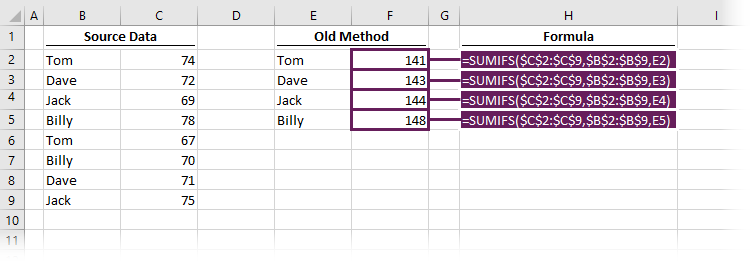
Cells F2-F5 each contain a formula. For example, F2 contains the following:
=SUMIFS($C$2:$C$9,$B$2:$B$9,E2)To calculate the result for each person, this formula would be copied down into the 3 rows below. In each formula, the last argument would change to reference cells E3, E4 and E5, respectively.
With dynamic arrays
But wait, the new Excel calculation engine returns multiple results from a single formula. Much like how our basic formula at the beginning of the post pushed results into other cells, SUMIFS works the same.
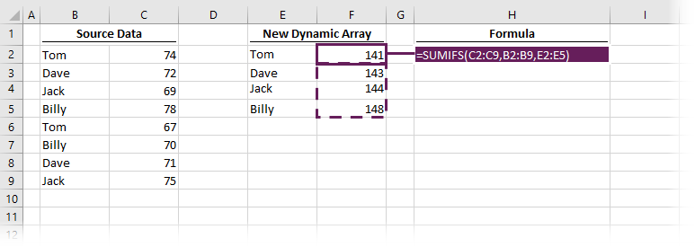
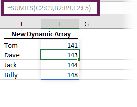
Rather than having 4 formulas, one for each cell; we can have one formula which returns results into 4 cells. The formula in cell F2 demonstrates this:
=SUMIFS(C2:C9,B2:B9,E2:E5)The last argument in the SUMIFS function is the value to be matched. Rather than one value, we provided an array of values to match in cells E2-E5. Therefore, Excel has performed all 4 calculations and spilled the results into cells F2-F5.
Which formulas spill?
So, which formulas spill, and which don’t? Good question. It depends on the arguments that the formula expects.
Basic aggregation functions, such as SUM, AVERAGE, MIN, MAX, etc., will not spill by themselves, which makes sense as they accept a range of values and only ever return a single value.
Generally, any function containing an argument in which a single value is evaluated expected is likely to spill. That single value has a technical term, it’s known as a scalar.
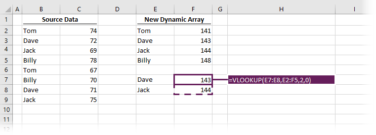
Let’s take VLOOKUP as an example. The first argument in VLOOKUP is the value to lookup, it’s generally a single value (it is a scalar). If we provide two or more values in that argument, the formula will spill, and calculate the result for each item included within the lookup value.
Look at the example below. The VLOOKUP in cell F7 is looking up Dave and Jack, so it calculates twice and returns the values in F7 and F8.
Generally, the rule is that If we’re working with standard formulas, then any time we use multiple scalars, it will spill. There are a few technical scenarios where this isn’t true, but that is outside the scope of this post.
Spilling
By clicking a formula or any cell in the spill range, a blue box is displayed to outline all the cells within the same spill range. Everything within the blue box is calculated by the top-left cell of that box.
By selecting any cell within the spill range, the formula bar displays the formula driving that result. If it is the top-left cell, we can edit the formula. However, if we select a cell, other than the top-left, the formula is greyed out and can’t be edited.
Look at the screenshot below; we have selected the second cell in the spill range. The formula is greyed out because it isn’t really in that cell, it’s in the top-left cell.
What happens if there is data already in the spill range? Will it overwrite the existing data? Thankfully, nothing too dramatic happens. Instead, the top-left cell returns a #SPILL! error.
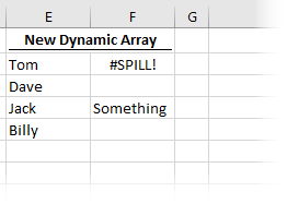
By clicking on the #SPILL! error, Excel displays a dotted line showing the spill range, and we can see what is causing the problem.
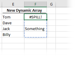
Then it’s your choice to (a) enter the formula in another location, or (b) move or delete the value causing the #SPILL! error.
#SPILL! errors occur in the following situations:
- The spill range is outside the available cells on the worksheet
- The spill range has an unknown size
- The dynamic array formula is included in an Excel table
- The spill range contains a merged cell
- The spill range is so large that Excel has run out of memory
# References
As a formula can spill results into other cells, we need a way to reference all the cells in the spill range. Thankfully, Microsoft has already thought of this and has created a new referencing methodology using the # symbol.
If the top-left cell in the spill range is in cell F2, we could reference the entire spill range by using F2#.
The screenshot below revisits our earlier example, but with an AVERAGE function added in cell F7.
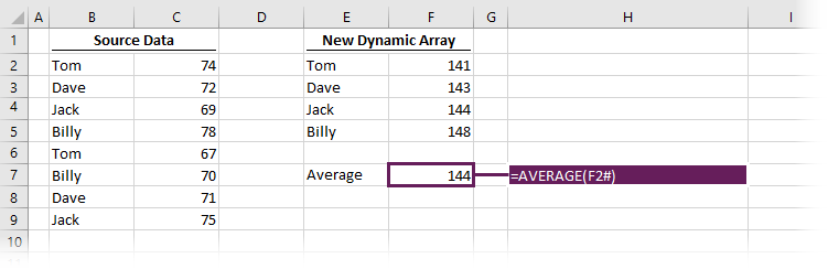
The formula in cell F7 is:
=AVERAGE(F2#)By using F2#, we are referencing all the cells in the spill range (cells F2, F3, F4 and F5). One significant advantage is that if the spill range changes size, the AVERAGE will automatically expand to include the increased range.
Constant arrays
Constant arrays have always existed in Excel; however, given the introduction of dynamic arrays, the use of constant arrays is likely to increase. They sound more complicated than they are. So, let’s just spend a few minutes understanding how they work.
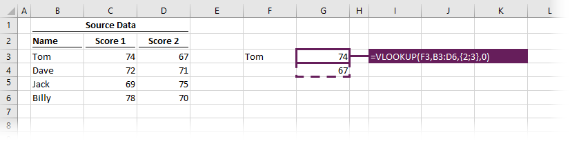
The easiest way to understand this is with an example; let’s use VLOOKUP.
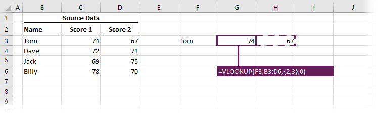
The formula in cell G3 is:
=VLOOKUP(F6,B2:D5,{2,3},0)This formula includes a constant array of {2,3}. Excel is using both values of 2 and 3 and spilling calculations for both into cell G3 and H3. The old method would require two formulas to achieve this, but with dynamic arrays we can use just one.
The two numbers in curly brackets are known as a constant array. See, they are not too scary after all.
With constant arrays, just be aware that columns are separated by commas and rows are separated by semi-colons. If we wanted to spill in rows instead of columns, we would use a semi-colon between the values (e.g., {2;3}).
=VLOOKUP(F6,B2:D5,{2;3},0)
If we were to enter the 2 and 3 in the opposite order (e.g. {3,2}), then the values returned would switch order too.
The @ symbol
To force Excel to operate in the old way, we can use the @ symbol. Let’s head back to our original example:
=B2:B6To use the old implicit intersection method which only returns the values that are in the same row, we can add the @ symbol.
=@B2:B6It’s unlikely that we would ever want to revert to the old way of calculating formulas. But initially, we are likely to see a lot of the @ symbol.
To ensure formulas built in previous versions of Excel continue to calculate the same result, the @ symbol will be added to some formulas automatically. This means that workbooks created in older versions of Excel but opened in the newer version of Excel should never spill. The @ symbol ensures backward compatibility.
NOTE: It may seem confusing because the @ symbol is already used within the structured referencing format that we use with Tables. But, if you think about it, in Tables, the @ symbol is used to reference items in the same row. Therefore, structured references in tables already have implicit intersection built in.
Conclusion
I’m sure you’ve got 100 questions spinning around your mind about dynamic arrays. There is a lot of new terminology and ways of working here. While the changes may seem confusing initially, you will soon see that this brings new powers to Excel users, which makes Excel easier to use.
Want to learn more?
There is a lot to learn about dynamic arrays and the new functions. Check out my other posts here to learn more:
- Introduction to dynamic arrays – learn how the excel calculation engine has changed.
- UNIQUE – to list the unique values in a range
- SORT – to sort the values in a range
- SORTBY – to sort values based on the order of other values
- FILTER – to return only the values which meet specific criteria
- SEQUENCE – to return a sequence of numbers
- RANDARRAY – to return an array of random numbers
- Using dynamic arrays with other Excel features – learn to use dynamic arrays with charts, PivotTables, pictures etc.
- Advanced dynamic array formula techniques – learn the advanced techniques for managing dynamic arrays
Discover how you can automate your work with our Excel courses and tools.
The Excel Academy

Make working late a thing of the past.
The Excel Academy is Excel training for professionals who want to save time.