
The SEQUENCE function is one of the new dynamic array functions that Microsoft released as part of introducing the dynamic arrays. This function makes use of changes to Excel’s calculation engine, which enables a single formula to display (or “spill” if using the new terminology) results in multiple cells. In the case of SEQUENCE, it will generate a list of sequential numbers in a two-dimensional array across both rows and columns.
At the time of writing, the SEQUENCE function is only available in Excel 2021, Excel 365 and Excel Online. It will not be available in Excel 2019 or earlier versions.
Table of Contents
Download the example file: Join the free Insiders Program and gain access to the example file used for this post.
File name: 0036 SEQUENCE Function in Excel.zip
Watch the video:

The arguments of the SEQUENCE function
The SEQUENCE function has four arguments; Rows, Columns, Start, Step.
=SEQUENCE(Rows, [Columns], [Start], [Step])
- Rows: The number of rows to return
- [Columns] (optional): The number of columns to return. If excluded, it will return a single column.
- [Start] (optional): The first number in the sequence. If excluded, it will start at 1.
- [Step] (optional): The amount to increment each subsequent value. If excluded, each increment will be 1.
Please note, while Excel creates sequences in rows and columns, it moves across columns, before moving down to the next row. Look at Example 3 to learn how to flip that functionality around.
Examples of using the SEQUENCE function
The following examples illustrate how to use the SEQUENCE function in Excel. As a dynamic array function, the result will automatically spill into neighboring rows and columns.
Example 1 – Basic Usage
The two examples below show the basic usage of the SEQUENCE function to provide a sequence of numbers.
Excluding optional arguments
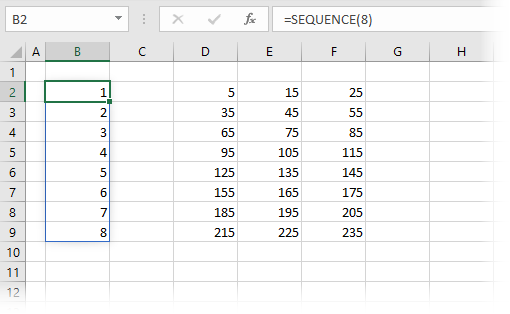
The formula in cell B2 is:
=SEQUENCE(8)In this formula, only the Rows argument is provided; all the other arguments ([Columns] optional, [Start] optional, and [Step] optional), have been excluded. Therefore, the default values are applied for each of these. SEQUENCE has created a list of sequential numbers; 8 rows, 1 column, starting at 1 and incrementing by 1 for each cell.
Including all arguments
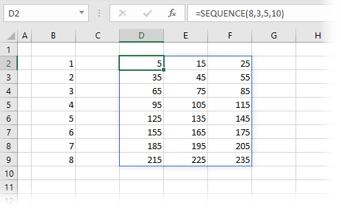
The formula in cell D2 uses all the arguments: Rows, Columns, Start and Step.
=SEQUENCE(8,3,5,10)When using the rows and columns arguments, it creates sequential numbers in a two-dimensional array. The formula is creating an array with:
- Rows argument = 8
- Columns argument = 3
- Start argument = 5
- Step argument = 10
The order of the numbers is important here, the function increments across the columns before moving to the next row.
Example 2 – Using SEQUENCE inside other functions
The example below shows how to use SEQUENCE inside the DATE function.
Note: As I am based in the UK, the screenshot below shows the UK date format (dd/mm/yyyy).
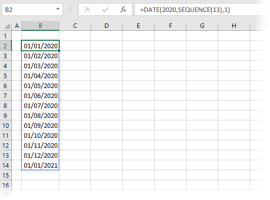
The formula in cell B2 is:
=DATE(2020,SEQUENCE(13),1)This formula creates a sequence of monthly dates starting on January 1st, 2020. The SEQUENCE function is applied to the month argument; therefore, it adds one to the month for each subsequent result. We have requested 13 months, but Excel is intelligent enough to know that 01/13/2020 doesn’t exist as a UK date format. Instead, the DATE function causes the result to roll-over into the next year and create 01/01/2021.
Example 3 – SEQUENCE row / column order
As already mentioned, the SEQUENCE formula in Excel creates sequential numbers across both rows and columns. However, by default they increment across columns before going down to the next row. To change this, we can use the TRANSPOSE function.
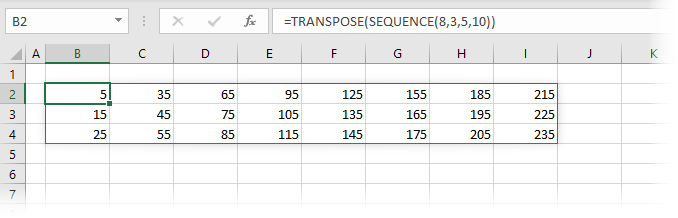
The formula in cell B2 is:
=TRANSPOSE(SEQUENCE(8,3,5,10))This is the same SEQUENCE function as we used in Example 1, but it has been wrapped in TRANSPOSE. Therefore, now the numbers increment down each row before going to the next column.
This can get a little confusing as while we have used the rows and columns arguments, the rows argument is displaying 8 columns and the column argument is displaying 3 rows. When we use this technique, we just need to remember that TRANSPOSE is applied as the last action.
Example 4 – Sequence with INDEX
The SEQUENCE formula in Excel is useful by itself, but when combined with other functions it’s power can be clearly seen.
In the screenshot below, we have a list of names and then the person’s ID or department. There are two rows for every individual. How can we get a list of just the ID’s sorted by last name? Let’s find out:
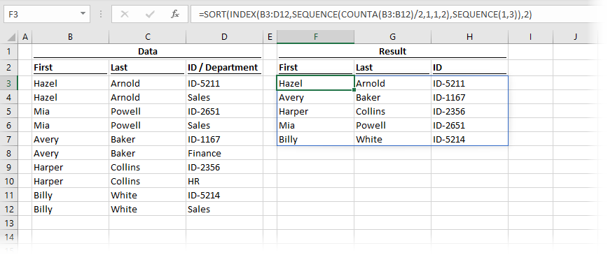
The formula in cell F2 is:
=SORT(INDEX(B3:D12,SEQUENCE(COUNTA(B3:B12)/2,1,1,2),SEQUENCE(1,3)),2)Let’s break this down:
- SEQUENCE(COUNTA(B3:B12)/2,1,1,2) – this part uses COUNTA to calculate the number of rows, then divides that by 2, as we want to return every 2nd row. SEQUENCE is then used to create the list which is 1 column, starts at the first row but steps by 2.
- SEQUENCE(1,3) – as we have 3 columns in our source, we want to return the same 3 columns. This creates the array list for INDEX to use.
- INDEX(B3:D12,…..) – The first SEQUENCE function above returns the value {1, 3, 5, 7, 9, 11}, the second SEQUENCE function above returns the values {1;2;3}. INDEX returns only the values from B3-B12 which are in these row and column positions.
- SORT(….,2) – finally the result is sorted by the 2nd column, which is the last name
This demonstrates the power of SEQUENCE as an enabler to more complex functions.
Example 5 – SEQUENCE in random order
Do you play bingo? No, me neither. But it creates an interesting example. I’m led to believe there are 75 numbers and those numbers can only appear once. By combining SORTBY, RANDARRAY and SEQUENCE we can put the sequence of 75 numbers into a random order (just like bingo).
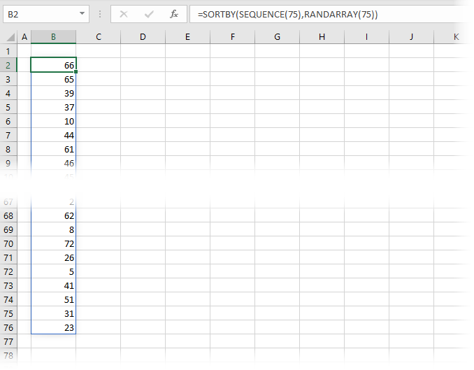
The formula in cell B2 is:
=SORTBY(SEQUENCE(75),RANDARRAY(75))The SEQUENCE function returns a list from 1 to 75. This list is sorted by another list of 75 random numbers created by RANDARRAY.
Other examples
The post about the SORT function also contains an example of using the SEQUENCE formula in Excel to create a list of the top 5 results.
Want to learn more?
There is a lot to learn about dynamic arrays and the new functions. Check out my other posts here to learn more:
- Introduction to dynamic arrays – learn how the excel calculation engine has changed.
- UNIQUE – to list the unique values in a range
- SORT – to sort the values in a range
- SORTBY – to sort values based on the order of other values
- FILTER – to return only the values which meet specific criteria
- SEQUENCE – to return a sequence of numbers in rows and columns
- RANDARRAY – to return an array of random numbers across a specific number of rows and columns
- Using dynamic arrays with other Excel features – learn to use dynamic arrays with charts, PivotTables, pictures etc
- Advanced dynamic array formula techniques – learn the advanced techniques for managing dynamic arrays
Discover how you can automate your work with our Excel courses and tools.
The Excel Academy

Make working late a thing of the past.
The Excel Academy is Excel training for professionals who want to save time.