FILTER function in Excel (How to + 8 Examples)

Filtering is a common everyday action for most Excel users. Whether using AutoFilter or a Table, it is a convenient way to view a subset of data quickly. Until the FILTER function in Excel was released, there was no easy way to achieve this with formulas. When Microsoft announced the changes to Excel’s calculation engine, they also introduced a host of new functions. One of those new functions is FILTER, which returns all the cells from a range that meet specific criteria.

At the time of writing, the FILTER function is only available in Excel 365, Excel 2021 and Excel Online. It will not be available in Excel 2019 or earlier versions.

Table of Contents

• Arguments of the FILTER function
• Examples of using the FILTER function
• Example 1 – FILTER returns an array of rows and columns
• Example 2 – #CALC! error caused by the FILTER function
• Example 3 – FILTER expands automatically when linked to a table
• Example 4 – Using FILTER with multiple criteria.
• Example 5 – Using FILTER for dependent dynamic drop-down lists
• Example 6 – Using FILTER with other functions
• Example 7 – Using FILTER to show matching items from a list
• Example 8 – Simulating wildcard search with FILTER

Watch the video:

Watch the video on YouTube

Arguments of the FILTER function

Before we look at the arguments required for the FILTER function, let’s look at a basic example to appreciate what it does.

Here the FILTER function returns all the values in cells B3-B10 where the number of characters is greater than 15. Not a scenario that many of us will need, but it perfectly demonstrates the power of the new FILTER function.

FILTER has three arguments:

=FILTER(array, include, [if_empty])

• array: The range of cells, or array of values to filter.
• include: An array of TRUE/FALSE results, where only the TRUE values are retained in the filter.
• [if_empty]: The value to display if no rows are returned.

Examples of using the FILTER function

The following examples illustrate how to use the FILTER function.

Example 1 – FILTER returns an array of rows and columns

In this example, cell F3 contains a single formula, but this formula returns an array of values into the neighboring rows and columns.

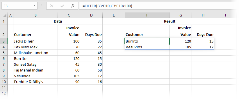
The formula in cell F3 is:

=FILTER(B3:D10,C3:C10>100)

This single formula is returning 2 rows and 3 columns of data where the values in C3-C10 are higher than 100.

Example 2 – #CALC! error caused by the FILTER function

The screenshot below displays what happens when the result of the FILTER function has zero results; we get the #CALC! error.

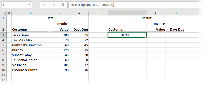
The formula in cell F3 is:

=FILTER(B3:D10,C3:C10>200)

As no rows meet the criteria of Invoice Value being higher than 200, the FILTER cannot return a value, so the #CALC! error is displayed.

Thankfully, Microsoft has given us the if_empty argument, which displays a message if there are no rows returned.

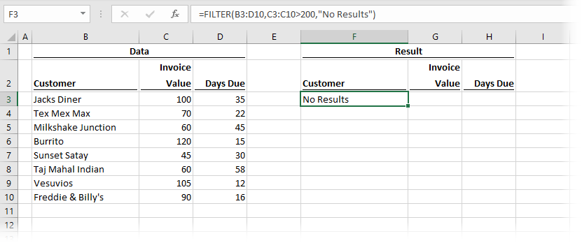
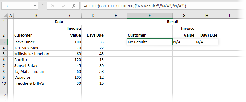
The formula in cell F3 is:

=FILTER(B3:D10,C3:C10>200,"No Results")

In the screenshot above, No Results displays instead of the #CALC! error.

If we wanted to display a result in each column, we could include a constant array within the if_empty argument. The following shows n/a in the Invoice Value and Days Due columns.

=FILTER(B3:D10,C3:C10>200,{"No Results","n/a","n/a"})

This formula would result in the following:

Example 3 – FILTER expands automatically when linked to a table

This example shows how the FILTER function responds when linked to an Excel table.

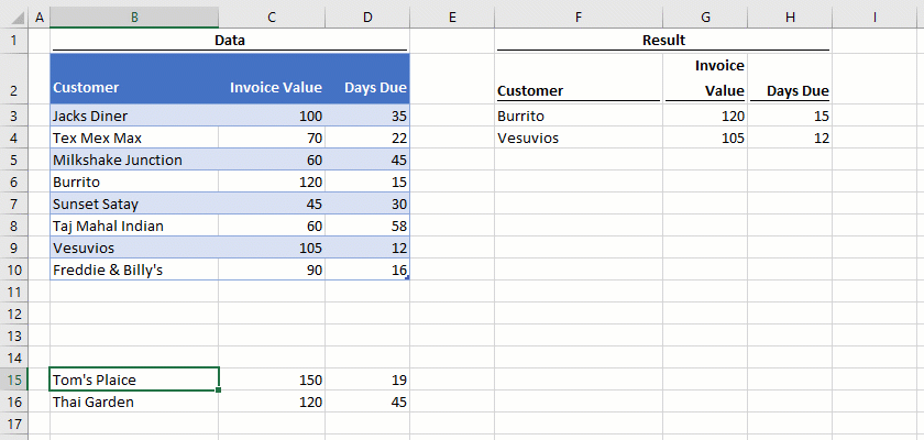
The FILTER is set to show items where Invoice Value is higher than 100. New records added to the Table which meet the criteria are automatically added to the spill range of the function. Amazing stuff!

Example 4 – Using FILTER with multiple criteria.

Example 4 shows how to apply FILTER with multiple criteria.

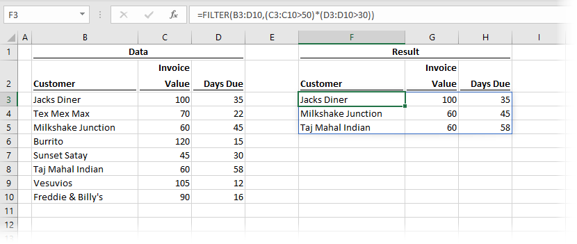
The formula in cell F3 is:

=FILTER(B3:D10,(C3:C10>50)*(D3:D10>30))

For anybody who has used the SUMPRODUCT function, this method of applying multiple conditions will be familiar. Multiplication creates AND logic (i.e., all the criteria must be TRUE). The example above shows where the Invoice Value is greater than 50 and the Days Due is greater than 30.

Addition creates OR logic (i.e., any individual condition can be TRUE).

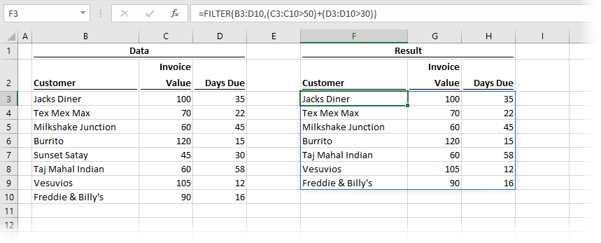
The formula in cell G3 is:

=FILTER(B3:D10,(C3:C10>50)+(D3:D10>30))

The example above shows where the Invoice Value is greater than 50 or the Days Due is greater than 30.

Example 5 – Using FILTER for dependent dynamic drop-down lists

Drop-down lists are a data validation technique. Dependent drop-down lists are an advanced technique where the lists change depending on the result of another cell. For example, if the first drop-down list displays country names, the second drop-down list should only display cities that exist in that country. In Excel 2019 and before there are only tedious methods to achieve this effect, but the new FILTER function makes this super easy.

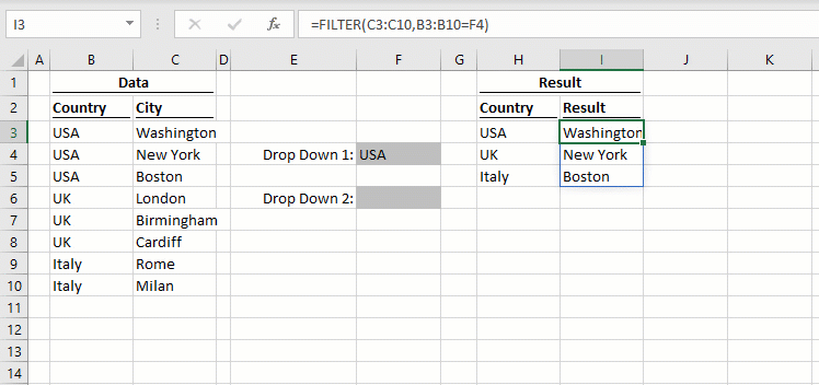
The formula in cell H3 is:

=UNIQUE(B3:B10)

The UNIQUE function creates a unique list to populate the drop-down in cell F4.

The formula in cell I3 is:

=FILTER(C3:C10,B3:B10=F4)

Depending on the value in cell F4, the values returned by the FILTER function change. The second drop-down in cell F6 changes dynamically based on the value in Cell F4.

Example 6 – Using FILTER with other functions

In this final example, FILTER is nested inside the SORT function.

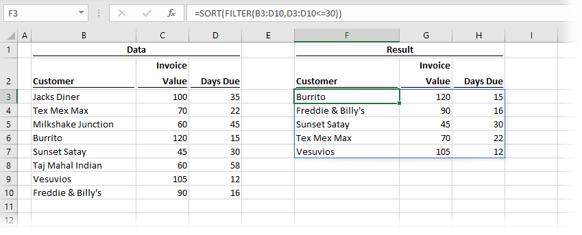
The formula in cell F3 is:

=SORT(FILTER(B3:D10,D3:D10<=30))

First, the FILTER function returns the cells based on the Days Due being less than or equal to 30. The SORT function then puts the Customers into ascending alphabetical order.

Example 7 – Using FILTER to show matching items from a list

How can we match a list of items that could have an unknown size? We can’t keep updating our FILTER function by adding and removing criteria. And, if we had a lot of items to match, it would soon become unmanageable. So, let’s see how we can solve this.

In the example below, the formula in cell H3 returns only the customers listed in F3:F4.

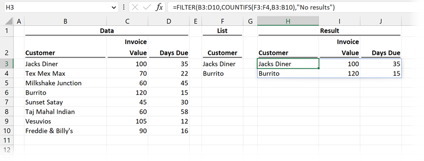
The formula in cell H3 is:

=FILTER(B3:D10,COUNTIFS(F3:F4,B3:B10),"No results")

The COUNTIFS function returns a positive number if the item exists in both the data and the list, or zero if it exists in only one. Since positive numbers are always TRUE and zeros are always FALSE, this provides the TRUE/FALSE logic required for the FILTER function to return only the matching items.

NOTE: If the list starting in F3 were generated by another array formula, or by Power Query this solution would be completely dynamic (that is outside the scope of the current post, so we have used static ranges for this example).

Example 8 – Simulating wildcard search with FILTER

The FILTER function does not allow wildcard characters in the criteria. However, by using a combination of SEARCH and ISNUMBER we can simulate a similar effect.

In the example below, the formula in cell H3 returns only the items where the customer name contains the letters in cell F3.

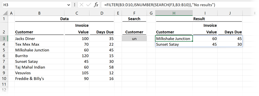
The formula in cell H3 is:

=FILTER(B3:D10,ISNUMBER(SEARCH(F3,B3:B10)),"No results")

SEARCH returns a number if the search term in cell F3 is found in each value in B3-B10.

ISNUMBER returns TRUE or FALSE for each value depending on if SEARCH returns a number. This TRUE/FALSE value provides the logic needed by FILTER to return the matching items.

In this scenario only, Milkshake Junction and Sunset Satay contain un as a substring, therefore only these customers are returned.

Want to learn more?

There is a lot to learn about dynamic arrays and the new functions. Check out my other posts here to learn more:

• Introduction to dynamic arrays – learn how the excel calculation engine has changed.
• UNIQUE – to list the unique values in a range
• SORT – to sort the values in a range
• SORTBY – to sort values based on the order of other values
• FILTER – to return only the values which meet specific criteria
• SEQUENCE – to return a sequence of numbers
• RANDARRAY – to return an array of random numbers
• Using dynamic arrays with other Excel features – learn to use dynamic arrays with charts, PivotTables, pictures etc.
• Advanced dynamic array formula techniques – learn the advanced techniques for managing dynamic arrays

---

What next?

Discover how you can automate your work with our Excel courses and tools.

The Excel Academy