
I can’t even begin to count the number of times I have created a unique list in Excel. I have performed it manually using remove duplicates from the ribbon, using PivotTables and with complex formulas, but that is now a thing of the past. When Microsoft announced changes to Excel’s calculation engine in September 2018, they also announced a host of new functions, one of which was the UNIQUE function in Excel.
At the time of writing, the UNIQUE function is only available for Microsoft 365, Excel Online and Excel 2021. It will not be available in Excel 2019 or earlier versions.
Table of Contents
Download the example file: Join the free Insiders Program and gain access to the example file used for this post.
File name: 0032 UNIQUE function in Excel.xlsx
Watch the video:

The arguments of the UNIQUE function
The UNIQUE function is straightforward to apply, as shown by the animation below.
UNIQUE has just three arguments. The last two are optional arguments and quite obscure, so you will only use them occasionally.
=UNIQUE(array, [by_col], [exactly_once])- array: the range or array to return values from.
- [by_col]: an optional argument where:
• FALSE = compare by row
• TRUE = compare by column.
If excluded, the argument defaults to FALSE. The impact of this is demonstrated in Example 4. - [exactly_once]: This argument depends on your interpretation of the word unique. If you want a list that includes only the items that appear once, then use TRUE for this argument. If you want a list that contains one instance of each item (i.e., a distinct list), then use FALSE. This is an optional argument and if excluded, will default to FALSE. The impact of this is demonstrated in Example 1.
Examples of using the UNIQUE function
The following examples illustrate how to use the UNIQUE function in Excel.
Example 1 – The difference between unique and distinct
The last argument of the UNIQUE function determines if it returns a distinct or unique list.
Distinct list
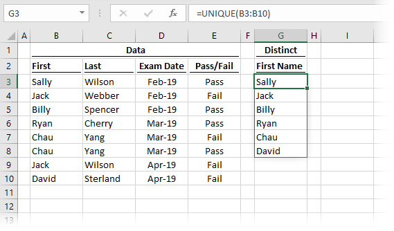
The formula in cell C3 is:
=UNIQUE(B3:B10)As the third argument has not been used, exactly_once has defaulted to FALSE and therefore shows a list of distinct results. Sally, Jack, Billy, Ryan, Chau and David all appear in cells B3-B10; therefore, we get a list of all those names.
Unique list (exactly once)
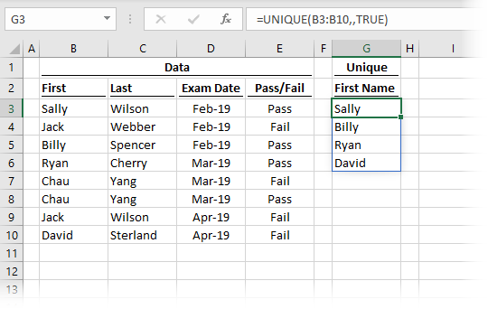
The formula in cell G3 is:
=UNIQUE(B3:B10,,TRUE)The third argument is TRUE, therefore UNIQUE return the results which appear only once in the array. Sally, Billy, Ryan, and David all appear only once within cells B3-B10. Jack and Chau appear twice and are therefore excluded from the result.
The difference between distinct and unique lists
When using the exactly_once argument, this is an important difference to understand:
- FALSE or empty = a distinct list
- TRUE = a list of items occurring only once
My guess is that in most situations, we will be using the distinct version of UNIQUE, which is the default option anyway.
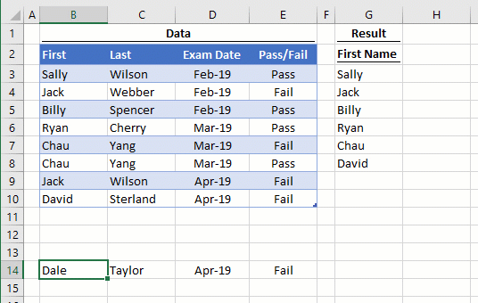
Example 2 – UNIQUE linked to an Excel table
Example 2 shows how UNIQUE responds when linked to an Excel table. When a new record is added, UNIQUE automatically expands to include the additional value in the spill range. Notice that the spill range of the UNIQUE function updates as soon as new items are added to the table.
The formula in cell G3 is:
=UNIQUE(tblExam[First])As the UNIQUE function is referencing the entire column, when the column expands or retracts, so does the result of the formula.
Example 3 – UNIQUE across multiple columns
UNIQUE is not restricted to a single column, it can assess the unique combination of multiple columns.
Method 1
This returns the unique list and retains the same number of columns as included in the first argument.
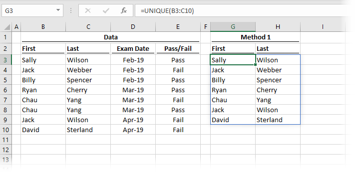
The formula in cell G3 is:
=UNIQUE(B3:C10)This includes the First and Last name columns in the array and returns both in the result. One instance of Chau Yang has been excluded as it appears twice in the source data.
Method 2
The second method uses functionality from the new calculation engine to concatenate columns before applying the UNIQUE function. As a result, only a single column of values is returned.
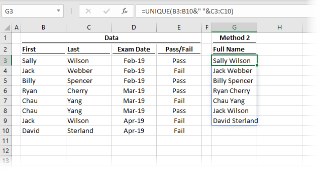
The formula in cell G3 is:
=UNIQUE(B3:B10&" "&C3:C10)Again, one instance of Chau Yang has been removed to provide a unique list within a single column.
Method 3
Sometimes we want a unique list with two columns that are not next to each other. In this circumstance, we can use the CHOOSE or CHOOSECOLS (only available in Excel 365) functions to reorder the columns.
The example below uses the CHOOSE function and is available in Excel 2021 and Excel 365.
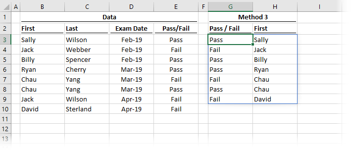
The formula in cell G3 is:
=UNIQUE(CHOOSE({1,2},E3:E10,B3:B10))By using CHOOSE, we have defined the first array as E3-E10 and the second array as B3-B10. These are the ranges that have been returned within the spill range.
If we have Excel 365 we could use either of the following alternative formulas which use CHOOSECOLS to achieve the same result:
=CHOOSECOLS(UNIQUE(B3:E10),4,1)=CHOOSECOLS(UNIQUE(B3:E10),{4,1})Example 4 – Using UNIQUE across columns
By default, Excel assumes UNIQUE should be applied on a vertical list. However, it can also work on a horizontal list.
Horizontal list
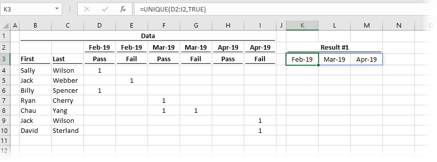
In the example above, cell K3 contains the following formula.
=UNIQUE(D2:I2,TRUE)The second argument in UNIQUE of [by_col] is set to TRUE. This tells the function that the data is in a horizontal format.
Use TRANSPOSE to convert horizontal & vertical (and vice versa)
If we had a vertical or horizontal list that we wanted to flip, we could use the TRANSPOSE function.
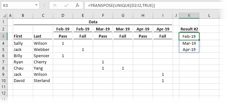
The formula in cell K3 is:
=TRANSPOSE(UNIQUE(D2:I2,TRUE))TRANSPOSE is used to change our horizontal UNIQUE list so the output is vertical.
Example 5 – Combining UNIQUE with SORT in a data validation list
Example 5 demonstrates how to combine the UNIQUE and SORT functions together.
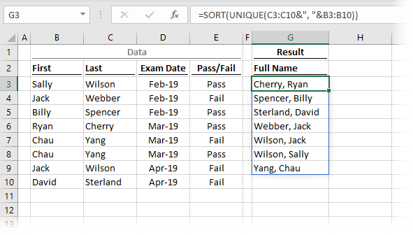
The formula in cell G3 is:
=SORT(UNIQUE(C3:C10&", "&B3:B10))The formula returns an alphabetically sorted unique list based on the Last and First names combined.
Often the purpose of a unique sorted list is for use within a data validation drop-down list. To do this, we can use the # symbol after the cell reference to refer to the entire spill range.
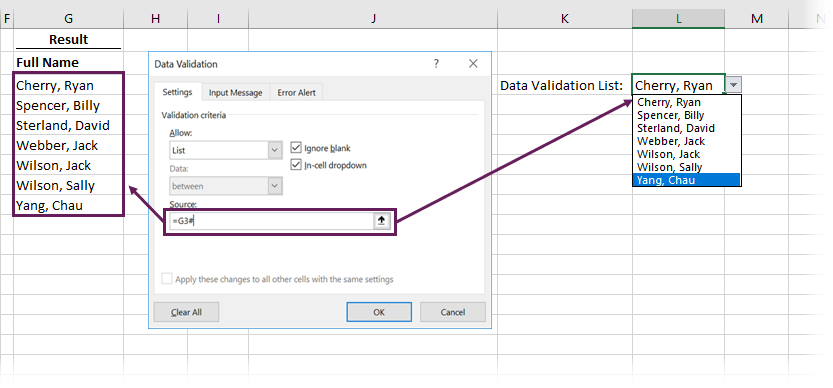
In the screenshot above, the formula is contained in cell G3. Therefore =G3# is used as the source for a data validation list. When the spill range increases or decreases in size, so does the drop-down list. It’s like magic!
Example 6 – Simple formula based Pivot Report
As a final example, we can create a simple Pivot Report using UNIQUE combined with some other common functions.
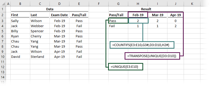
The formula in cell G3 is:
=UNIQUE(E3:E10)This is the standard UNIQUE function applied to the Pass/Fail column.
The formula in cell H2 is:
=TRANSPOSE(UNIQUE(D3:D10))TRANSPOSE switches the output of UNIQUE from displaying in rows to displaying in columns. The 3 distinct dates in the Exam Date column are now listed as column headers.
The formula in H3 is:
=COUNTIFS(E3:E10,G3#,D3:D10,H2#)The COUNTIFS function includes the # references, so it automatically spills in the same way as the cells it is dependent upon.
With these 3 simple formulas, we have created a complete report – amazing! Remember, if the source is an Excel table, the output will expand as new data is added – even more amazing!!
Want to learn more?
There is a lot to learn about dynamic arrays and the new functions. Check out our other posts here to learn more:
- Introduction to dynamic arrays – learn how the excel calculation engine has changed.
- UNIQUE – to list the unique values in a range
- SORT – to sort the values in a range
- SORTBY – to sort values based on the order of other values
- FILTER – to return only the values which meet specific criteria
- SEQUENCE – to return a sequence of numbers
- RANDARRAY – to return an array of random numbers
- Using dynamic arrays with other Excel features – learn to use dynamic arrays with charts, PivotTables, pictures etc.
- Advanced dynamic array formula techniques – learn the advanced techniques for managing dynamic arrays
Discover how you can automate your work with our Excel courses and tools.
The Excel Academy

Make working late a thing of the past.
The Excel Academy is Excel training for professionals who want to save time.