VLOOKUP: Lookup the nth item (without helper columns)

In this series, Mastering VLOOKUP we have covered a lot of ground. But this post is one of the most fiendish of all. VLOOKUP, by its design, is intended to return the first match it finds. But, if we want the 2nd, 3rd or nth VLOOKUP it not so easy. Often people resort to helper columns, but that’s really not necessary (and nowhere near as much fun!)

Finding the nth Lookup

Look at the screenshot below. Our data is sorted into age order, but how could we find the find the age of the 3rd Dave in the list?

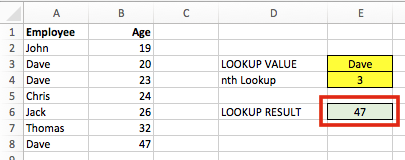
The formula in cell E6 is:

{=VLOOKUP(SMALL(IF(A2:A8=E3,ROW(A2:A8)),E4),CHOOSE({1,2},
ROW(A2:A8),B2:B8),2,0)}

Firstly – this is an array formula. Don’t type the { } at the start and the finish, but enter the formula with Ctrl+Shift+Enter and Excel will add them automatically.

Secondly – yes, this formula is scary! But stick with me, I’ll do my best to explain it.

How does the formula work?

The key to this formula working correctly in the SMALL function along with the ROW function. Let’s build up the formula bit by bit.

IF Function

{=VLOOKUP(SMALL(IF(A2:A8=E3,ROW(A2:A8)),E4),CHOOSE({1,2},
ROW(A2:A8),B2:B8),2,0)}

The red highlighted section is almost a standard IF function. However, it is working on a range of cells, rather than a single cell. If any cells in A2-A8 equals the lookup value, Dave in our example, the row number of that cell is returned. If the name is not Dave then FALSE is returned. The name Dave is in Row 3, Row 4 and Row 8, so the IF function would return an array of {FALSE, 3, 4, FALSE, FALSE, FALSE, 8}.

SMALL Function

{=VLOOKUP(SMALL(IF(A2:A8=E3,ROW(A2:A8)),E4),CHOOSE({1,2},
ROW(A2:A8),B2:B8),2,0)}

We have wrapped the result of the IF function in the SMALL function. Cell E4 is the nth value which we are searching for. In our example E4 is 3, as we are looking for the 3rd lookup. This will now look for the 3rd smallest value from the IF function array returned above. The 3rd smallest result from the array is 8; {FALSE,3,4,FALSE,FALSE,FALSE,8}.

This completes the first argument of the VLOOKUP function; the lookup value is 8. Even though we are searching for the 3rd VLOOKUP of Dave, the 3rd Dave is in the 8th row. So, we are looking up 8. Hopefully that’s not too confusing.

CHOOSE Function

The CHOOSE function operates in a similar way as we encountered when doing a VLOOKUP to the left. However, we will be using the row number as the lookup column.

Within the CHOOSE function the numbers within the { } determine which column is which.

{=VLOOKUP(SMALL(IF(A2:A8=E3,ROW(A2:A8)),E4),CHOOSE({1,2},
ROW(A2:A8),B2:B8),2,0)}

Column 1, the lookup column, is just the row number. This would return an array of {2, 3, 4, 5, 6, 7, 8}. Our lookup value is 8, so our VLOOKUP will be able to find a value.

{=VLOOKUP(SMALL(IF(A2:A8=E3,ROW(A2:A8)),E4),CHOOSE({1,2},
ROW(A2:A8),B2:B8),2,0)}

Column 2 is defined as B2-B8.

VLOOKUP Function

{=VLOOKUP(SMALL(IF(A2:A8=E3,ROW(A2:A8)),E4),CHOOSE({1,2},
ROW(A2:A8),B2:B8),2,0)}

The VLOOKUP function is used the undertake an exact match of Row number 8 and return the value from Column 2 (Cells B2-B8).

The Result

The result of our formula is 47. We can adapt this formula to find the nth lookup from any data set.

It was tough going there for a while, but hopefully you’ve made it through.

A few comments/pointers

Is there a more efficient way?

Yes, there is. Once we have obtained the row number of a matching value it would probably be easier to apply an INDEX formula, rather than a VLOOKUP. But the point is that VLOOKUP a possible option. If VLOOKUP is one of the few functions you know, then it use it.

Spacer Characters

We could/should use spacer characters in this formula. Whilst it is very unlikely to return an incorrect result with our example, it could be possible with other data sets, so best to use spacer characters. Given the complexity of the example, I decided to leave them out. If we wanted them the formula would be:

{=VLOOKUP(E3&"^"&SMALL(IF(A2:A8=E3,ROW(A2:A8)),E4),
CHOOSE({1,2},A2:A8&"^"&ROW(A2:A8),B2:B8),2,0)}

Helper Columns

If this example seems too complex they the easier option is just to use a helper column.

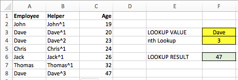
The formula in B2 is:

=A2&"^"&COUNTIF($A$2:A2,A2)

Copy this formula down to B8. Then the formula in F6 could be:

=VLOOKUP(F3&"^"&F4,B2:C8,2,0)

Simple.

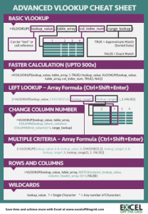
Download the Advanced VLOOKUP Cheat Sheet

Download the Advanced VLOOKUP Cheat Sheet. It includes most of the tips and tricks we’ve covered in this series, including faster calculations, multiple criteria, left lookup and much more.

Please download it and pin it up at work, you can even forward it onto your friends and co-workers.