
Most Excel users think that VLOOKUP can only be used with a single criterion; until a few months ago I believed this was also the case. In the past I had used INDEX/MATCH or helper columns because I had not appreciated how much could be achieved with the VLOOKUP & CHOOSE combination. We have already looked at this combination when discovering how to VLOOKUP to the left. But, as you will see, we can take this combination even further.
VLOOKUP & CHOOSE Combination
Let’s start with a basic example. You work for a company with the following telephone list:
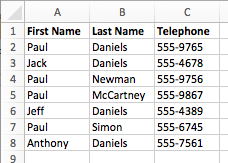
Wow! There are lots of people with the first name Paul, and lots of people with the last name of Daniels – that’s funny, what are the chances? Then your manager asks you to create a spreadsheet, in which you will need to look up the telephone number of certain individuals. Suddenly, the repetition of the names is not funny, it is now very painful. How will you be able to separate all of the Paul’s and all of the Daniel’s?
VLOOKUP to the rescue!!!
We can still use a VLOOKUP formula in this scenario to return the value. Seriously we can!
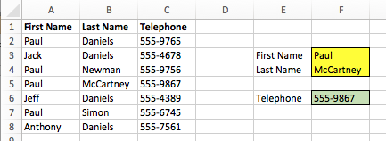
The formula in cell F6 is returning a lookup to both Column A and Column B to find the telephone number for Paul McCartney. The formula in this cell is:
{=VLOOKUP(F3&"^"&F4,CHOOSE({1,2},A2:A8&"^"&B2:B8,C2:C8),2,FALSE)}
Using this formula, it is possible to lookup the First Name and Last Name to return the Telephone Number. This is an Array formula – which means the formula is entered without { } at the start and end of the formula (we still enter the { } in the middle). Pressing Ctrl+Shift+Enter will enter the formula, and Excel will automatically add { } to the start and end of the formula.
How does the VLOOKUP & CHOOSE (Array) combination work?
Let’s break this formula down into separate chunks.
{=VLOOKUP(F3&"^"&F4,CHOOSE({1,2},A2:A8&"^"&B2:B8,C2:C8),2,FALSE)}
The sections highlighted above are the standard VLOOKUP formula which we know. The only difference is, cells F3 and F4 are being combined with a spacer character. The result of F3&”^”&F4 is “Paul^McCartney”
{=VLOOKUP(F3&"^"&F4,CHOOSE({1,2},A2:A8&"^"&B2:B8,C2:C8),2,FALSE)}
The section highlighted above is indicating that column 1 for the VLOOKUP should be the combination of column A and column B separated by a spacer character. As this is an Array formula this section creates a temporary range of values which would be as follows.
Row 2= “Paul^Daniels”
Row 3= “Jack^Daniels”
Row 4= “Paul^Newman”
Row 5= “Paul^McCartney”
Row 6= “Jeff^Daniels”
Row 7= “Paul^Simon”
Row 8= “Anthony^Daniels”
Assuming a match is found (row 5 in our example), it will then return the value from column 2.
{=VLOOKUP(F3&"^"&F4,CHOOSE({1,2},A2:A8&"^"&B2:B8,C2:C8),2,FALSE)}
In our CHOOSE formula, column 2 is defined as being cells C2-C8. Therefore, Paul McCartney’s telephone number is returned as 555-9867
Notes & comments
Here are some things to be aware of:
- It is possible to use this formula with other techniques presented in this Mastering VLOOKUP Series (such as the double VLOOKUP method for faster calculations)
- If you click back into the formula and do not enter it with Ctrl+Shift+Enter then an error will be displayed. You must Ctrl+Shift+Enter every time.
- Of all the multiple criteria lookup methods this is one of the lowest to calculate.
For other examples of the VLOOKUP & CHOOSE combination read “How the VLOOKUP to the left“
Summary
Once again VLOOKUP proves itself to be more diverse than it may first appear. By mastering this technique you will be able to do things with VLOOKUP which most Excel users can only dream of.
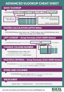
Download the Advanced VLOOKUP Cheat Sheet
Download the Advanced VLOOKUP Cheat Sheet. It includes most of the tips and tricks we’ve covered in this series, including faster calculations, multiple criteria, left lookup and much more.
Please download it and pin it up at work, you can even forward it onto your friends and co-workers.
Download the example file: Join the free Insiders Program and gain access to the example file used for this post.
File name: 0166 Advanced VLOOKUP.pdf
Other posts in the Mastering VLOOKUP Series
- How to use VLOOKUP
- VLOOKUP: What does the True/False statement do?
- VLOOKUP: How to calculate faster
- How to VLOOKUP to the left
- VLOOKUP: Change the column number automatically
- VLOOKUP with multiple criteria
- Using wildcards with VLOOKUP
- How to use VLOOKUP with columns and rows
- Automatically expand the VLOOKUP data range
- VLOOKUP: Lookup the nth item (without helper columns)
- VLOOKUP: List all the matching items
- Advanced VLOOKUP Cheat Sheet
Discover how you can automate your work with our Excel courses and tools.
The Excel Academy

Make working late a thing of the past.
The Excel Academy is Excel training for professionals who want to save time.
Are there any named ranges “1” and “2” to make this formula work?
Hi Daniel – that’s an interesting idea, you certainly could use named ranges. Though you would not be able to call them “1” and “2”, as they are not valid names for a named range.