
Unfortunately, VLOOKUP, whilst powerful, simple and easy to use, is one of the least flexible functions in Excel. Just imagine for a moment that we have entered the following formula into Cell E6 (see screenshot below).
=VLOOKUP(E4,A2:B10,2,0)
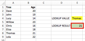
This formula is returning the value from the 2nd column (Column B) – result 21.
But, what happens when a column is inserted between Column A and Column B? The Range A2:B10 will automatically update to become A2:C10, but the lookup column number will remain the same. The value will still be returned from the 2nd column, even though that is no longer the column we wish to return the value from.
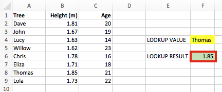
The result has now changed to 1.85, rather than 21.
Assuming we noticed, we now need to go back through each of the VLOOKUP formulas to change the 2 to a 3. Painful!
We tend to include the column number as a hard-coded number. But if we can create the column number using formulas then VLOOKUP will be able to update itself when additional columns are inserted.
Using the COLUMN formula
The COLUMN() formula will return the column number for the cell which it is referring to. Here are some examples:
=COLUMN(G2)
This will return 7, because G is the 7th column
=COLUMN(Z12)
This will return 26, because Z is the 26th column
COLUMN only calculates based on the cell reference provided. By creating a formula using two COLUMN functions we can calculate the column number required. The format of the formula is:
=COLUMN([lookup return column])-COLUMN([first column])+1
Where [first column] and [lookup return column] are the cell references to any cell in that column. Using our initial example, it would be as follows
=COLUMN(B1)-COLUMN(A1)+1
Try it out – this gives us a result of 2. Now we can replace the column number in our original VLOOKUP function as follows:
=VLOOKUP(E4,A2:B10,COLUMN(B1)-COLUMN(A1)+1,0)
If any columns between Column A and Column B are inserted, our entire formula will update itself and still return the correct values.
=VLOOKUP(E4,A2:C10,COLUMN(C1)-COLUMN(A1)+1,0)
Other advantages of using COLUMN in VLOOKUP
This method of using the COLUMN formula has one other big advantage; the formula can now be dragged, copied and moved.
=VLOOKUP(E$4,$A$2:$B$10,COLUMN(B$1)-COLUMN($A$1)+1,0)
By inserting the $ signs into the right places, the column number will change as the formula is copied across.
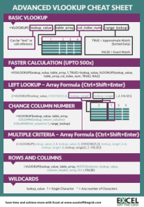
Download the Advanced VLOOKUP Cheat Sheet
Download the Advanced VLOOKUP Cheat Sheet. It includes most of the tips and tricks we’ve covered in this series, including faster calculations, multiple criteria, left lookup and much more.
Please download it and pin it up at work, you can even forward it onto your friends and co-workers.
Download the example file: Join the free Insiders Program and gain access to the example file used for this post.
File name: 0166 Advanced VLOOKUP.pdf
Other posts in the Mastering VLOOKUP Series
- How to use VLOOKUP
- VLOOKUP: What does the True/False statement do?
- VLOOKUP: How to calculate faster
- How to VLOOKUP to the left
- VLOOKUP: Change the column number automatically
- VLOOKUP with multiple criteria
- Using wildcards with VLOOKUP
- How to use VLOOKUP with columns and rows
- Automatically expand the VLOOKUP data range
- VLOOKUP: Lookup the nth item (without helper columns)
- VLOOKUP: List all the matching items
- Advanced VLOOKUP Cheat Sheet
Thank you for the help. I really appreciate it !!
If helpful to you, I prefer the below method instead of the column function described here.
index(results column, match(lookup value, search column,0))
If you do change your suggested solution, there is no need to thank me or give credit to me.
Cheers,
Andrew
Hi Andrew – yes, I completely agree. I even wrote an extensive post about it:
https://exceloffthegrid.com/real-reason-index-match-better-vlookup/
Unfortunately, not everybody is a fan of INDEX/MATCHs, VLOOKUP continues. But there is the new XLOOKUP function which may be the best option yet.