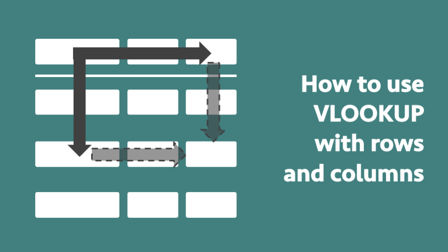
There are times when our data is laid out in columns and rows. In these circumstances, we may need to VLOOKUP row and column at the same time.
Look at the example below, how can we look up the Low for Jun? This post will show you how.
VLOOKUP row and column with VLOOKUP & MATCH
By combining the VLOOKUP function with the MATCH function, we can achieve a lookup to a row and a column at the same time; this is often referred to as a two-way lookup.
MATCH
The MATCH function is a very useful; it returns the position of a lookup value within a range.
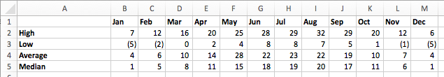
Using our example data; we can find the column number of “Jun” using the Match function.
=MATCH("Jun",B1:M1,0)
The result of this formula is 6, as in the Range B1-M1 “Jun” is the 6th item. If we were to look up “Nov”, this would return 11, as that is the 11th item.
The last argument in the MATCH function is important. We will be using 0 as that will provide an exact match.
VLOOKUP & MATCH together
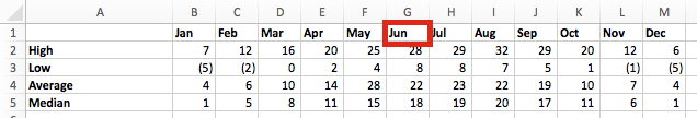
We can insert MATCH into the VLOOKUP function in place of the column number.
The VLOOKUP function counts the first column as 1, but our MATCH function starts at column B, so it is necessary to add 1 to the column number for the VLOOKUP to return the value from the correct column.
The formula in B12 is as follows:
=VLOOKUP(B9,A2:M5,MATCH(B10,B1:M1,0)+1,FALSE)
Looking up multiple rows
We’ve seen, in previous posts, that it is possible to use VLOOKUP with multiple criteria where the data is in two or more columns. But what if we want to match multiple rows?
The example below shows July appearing twice in our data, once for 2016 and once for 2017. By making the MATCH formula an array formula we can match the two column criteria of month and year together.
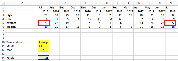
The formula in cell B14 is:
{=VLOOKUP(B10,A3:N6,MATCH(B11&"^"&B12,B1:N1&"^"&B2:N2,0)+1,FALSE)}
This formula is starting to look a bit complicated now, so let’s break it down.
Firstly, this is an array formula. Type the formula into Excel without the { }, but press Ctrl+Alt+Enter to enter the formula. Excel will then add the { } by itself automatically.
{=VLOOKUP(B10,A3:N6,MATCH(B11&"^"&B12,B1:N1&"^"&B2:N2,0)+1,FALSE)}
Secondly, let’s just look at the first argument of the MATCH function. This is simply combining the values of “Jul” and “2016” together with a spacer character in the middle.
{=VLOOKUP(B10,A3:N6,MATCH(B11&"^"&B12,B1:N1&"^"&B2:N2,0)+1,FALSE)}
The next argument of the MATCH function creates a temporary array of values with a spacer character in the middle. This only works because it is an array formula.
{=VLOOKUP(B10,A3:N6,MATCH(B11&"^"&B12,B1:N1&"^"&B2:N2,0)+1,FALSE)}
The temporary array would include the following {“Jul^2016” , “Aug^2016” , “Sep^2016” , “Oct^2016” […all the way up to…] “Jun^2017” , “Jul^2017”}
The lookup value in the MATCH function is compared to this temporary array. Provided the year and the month match a value will be returned. By changing the year in cell B12 the value from N5, rather than B5 will be returned. The image below shows the result as 27, rather than 23.

Multiple condition rows and columns
If you ever need to match multiple condition rows and multiple condition columns together, then it’s probably best to consider the INDEX/MATCH/MATCH formula. As I’m not sure it’s possible to push the VLOOKUP formula that far.
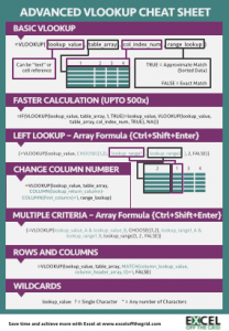
Download the Advanced VLOOKUP Cheat Sheet
Download the Advanced VLOOKUP Cheat Sheet. It includes most of the tips and tricks we’ve covered in this series, including faster calculations, multiple criteria, left lookup and much more.
Please download it and pin it up at work, you can even forward it onto your friends and co-workers.
Download the example file: Join the free Insiders Program and gain access to the example file used for this post.
File name: 0166 Advanced VLOOKUP.pdf
Other posts in the Mastering VLOOKUP Series
- How to use VLOOKUP
- VLOOKUP: What does the True/False statement do?
- VLOOKUP: How to calculate faster
- How to VLOOKUP to the left
- VLOOKUP: Change the column number automatically
- VLOOKUP with multiple criteria
- Using wildcards with VLOOKUP
- How to use VLOOKUP with columns and rows
- Automatically expand the VLOOKUP data range
- VLOOKUP: Lookup the nth item (without helper columns)
- VLOOKUP: List all the matching items
- Advanced VLOOKUP Cheat Sheet<
Discover how you can automate your work with our Excel courses and tools.
The Excel Academy

Make working late a thing of the past.
The Excel Academy is Excel training for professionals who want to save time.
I simply want to transcribe column inputs into rows. So for example, want to transcribe values in rows a1 to a10 into columns m4 to v4
What lookup command and formula would do that?
Thank you.
Hi Michael
You should look at the TRANSPOSE function, or if that’s not flexible enough, the OFFSET function.
Yes, I figured that out. Thank you, it is always good to know someone who knows so much about Excel.