Have you heard of the mysterious “array formulas”? Do you use them? Or are you like most Excel users, you’ve placed them in the “too hard” pile, never to be seen again. They always seem to crop up in forums as solutions to some tricky formula questions.
In this post, I want to introduce to you one type of array formula which is actually pretty easy to understand and can be applied to lots real-life situations. Once you’ve grasped the concept of this type of array formula, you’ll be able to apply it over and over again. Your work colleagues will look at you like you’re an Excel genius, they will be mesmerized by the apparently impossible calculation you’ve just performed . . . but secretly you’ll know it wasn’t that difficult.
Array formula basics
An array formula is a calculation which works with an array or series of data. Don’t worry if that concept blows your mind at the moment, by the end of this post it’ll hopefully make sense.
Often array formulas are entered by pressing Ctrl + Shift + Enter – hence why they are sometimes referred to as CSE formulas. There are array functions which do not require Ctrl + Shift + Enter to be used. So, just be aware that Ctrl + Shift + Enter does not apply to all array formulas.
The type of array formula we will be using in this example does require Ctrl + Shift + Enter. Once the formula has been entered into the formula bar, do not just press Enter, but press Ctrl + Shift + Enter at the same time. You will know when it has worked because Excel will automatically show a ” { ” (opening curly bracket) at the start of the formula and a ” } ” (closing curly bracket) at the end of the formula.
You must press Ctrl + Shift + Enter, not just when creating the formula the first time, but anytime you edit the formula.
In the examples below I will show the { } curly brackets, but remember, don’t type these, Excel will display these by itself.
Basic array formula example
For our example, we will be looking at the type of array formula which returns the result into a single cell.
We are going to recreate the SUMIF function as an array formula. Why? Hopefully you already understand the SUMIF function, so the concepts will be easier to understand. The goal is not to recreate a SUMIF using an array formula, but to learn the concepts so you can apply it to your own scenarios.
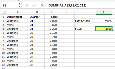
Look at the table of data below, it shows the quarterly sales for 3 departments of a clothing store. If we wanted to know the annual total for any department we could use the SUMIF function.

The value in Cell F4 is calculating the total sales for the Men’s clothing department:
=SUMIF(A2:A13,F2,C2:C13)
Let’s break down the SUMIF function down into its two parts SUM and IF. Logic requires that the IF function must be calculated first, then the SUM function can be used to calculate the total. This is what we will do.
The first step to convert SUMIF into an array formula is to create an IF function for a single row.
=IF(A2=F2,C2,0)
The second step is to expand the range to include all the cells required for the calculation (this is what makes this an array formula, as it calculates based on an array of cells).
=IF(A2:A13=F2,C2:C13,0)
The third step is to include the SUM function around the IF function.
=SUM(IF(A2:A13=F2,C2:C13,0))
The final step is to press Ctrl + Shift + Enter to enter the formula (notice that Excel displays the { } by itself).

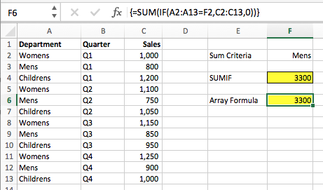
The formula in Cell F6 is:
{=SUM(IF(A2:A13=F2,C2:C13,0))}
You have just created an array formula. That wasn’t so hard, was it.
Understanding the calculation
Let’s briefly understand why this formula works.
{=SUM(IF(A2:A13=F2,C2:C13,0))}
The section of the formula in blue above will calculate as TRUE or FALSE for each cell. Does A2 = F2, then does A3 = F2, then does A4 = F2, and so on. As F2 is a single cell this is used as a comparison for every cell in A2 – A13.
There are 12 cells in the range, so there are 12 TRUE/FALSE results.
{=SUM(IF({FALSE;TRUE;FALSE;FALSE;TRUE;FALSE;FALSE;TRUE;FALSE;FALSE;TRUE;FALSE},
C2:C13,0))}
The orange section in the formula above is will calculate as shown below.
{=SUM(IF({FALSE;TRUE;FALSE;FALSE;TRUE;FALSE;FALSE;TRUE;FALSE;FALSE;TRUE;FALSE},
{1000;800;1200;1100;750;1050;1150;850;950;1250;900;1000},0))}
Each of these formula results is calculated as a separate IF function.
{=SUM(IF({FALSE;TRUE;FALSE;FALSE;TRUE;FALSE;FALSE;TRUE;FALSE;FALSE;TRUE;FALSE},
{1000;800;1200;1100;750;1050;1150;850;950;1250;900;1000},0))}
The first IF function has calculated as FALSE, therefore the result will be zero (it would have been 1000, if it were TRUE)
{=SUM(IF({FALSE;TRUE;FALSE;FALSE;TRUE;FALSE;FALSE;TRUE;FALSE;FALSE;TRUE;FALSE},
{1000;800;1200;1100;750;1050;1150;850;950;1250;900;1000},0))}
The second IF function has calculated as TRUE, therefore the result will be 800 (it would have been zero if it were FALSE)
This continues for each result of the IF function. This calculates down to provide the following result.
{=SUM({0;800;0;0;750;0;0;850;0;0;900;0}))}
This is now a straightforward SUM function, which will add the numbers together. The result is 3,300 (which is exactly the same as SUMIF).
Applying the array formula concept
This concept works for a variety of situations. Now that you know the concept, you could create your own complex formulas, which would be impossible with a normal function.
You could create a SUMIFBUTFIXEDVALUEIFNOT (Sum if, but fixed value if not) function:
{=SUM(IF(A2:A13=F2,C2:C13,500))}
Or Maybe the AVERAGEROWNUMBER (average row number) function:
=AVERAGE(ROW(A2:A13))
You can also create the benefit of helper columns without needing to actually create a helper column. In the example below Cells E14 & F14 are combined into a single search criterion then compared to A2 & B2 combined, then A3 & B3 combined, then A4 & B4 combined, and so on.
=MATCH(E14&F14,A2:A13&B2:B13,0)
Warnings
Array formulas may sound great, but there are some issues to be aware of:
- They can be very slow to calculate, and they are often much slower than using a helper column
- Most people won’t understand your work (though this may be a good thing)
- If Ctrl + Shift + Enter is not used, it is likely to display either #VALUE or worse an incorrect result
Other examples of array formulas
Here are some posts from the blog which include other examples of array formulas.
- Create a Top 10 using formulas
- VLOOKUP: list all the matching items
- VLOOKUP: Lookup the nth item (without helper columns)
- VLOOKUP with multiple criteria
- How the VLOOKUP to the left
Discover how you can automate your work with our Excel courses and tools.
The Excel Academy

Make working late a thing of the past.
The Excel Academy is Excel training for professionals who want to save time.


I get most use out of array formulas with MAX and MIN functions, such as finding the max and min of a dataset if certain conditions are met. To your point about slowness – this has always been a big issue for me. Speed is not only hindered based on the number of formulas you have, but also the size of the dataset they reference. I frequently find myself moving to VBA for anything that may scale up at some point in the future.
Hi Rob,
With the introduction of MAXIFS and MINIFS in Excel 2016 I think there will be less need for MAX and MIN with array formulas in the future.
I certainly agree that VBA can be an option when speed becomes an issue, but that can bring its own challenges. I think more tools we have at our disposal the more we can pick and choose based on each scenario.
The skills of those people that are users of Excel do not have to be greater than what they need in their work. I suspect that >95% of users need only rudimentary Excel skills. Those who can understand array formulas are likely <1% of users.
Hi David,
Firstly, apologies for the late reply to this, I’ve only just seen it. You’re right, most users will never need to touch an array formula.
They appear to have a stigma about them, that they are too hard to learn. This isn’t true of all array formulas, some are quite simple. It’s the 1% who could benefit from having it in their Excel ‘toolkit’.
Also, understanding the concepts helps us to think about data and Excel differently, so the benefits are wider reaching than just array formulas. This could also benefit the 1%.