How to use Table slicers for advanced interactivity in Excel

Having looked at how to use slicers with PIVOTBY and FILTER in a previous post. Let’s take this a step further and discover how we can use Table slicers for more advanced user interactivity.

Table of Contents

• Example
• Getting the table slicer selections
• Changing and applying table slicer selections
• Disconnected slicers
• Slicer selections LAMBDA
• Conclusion

Watch the video

Watch the video on YouTube

Example

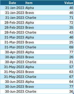
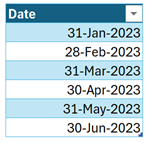
The data for our example is straightforward. The Data table has 3 columns: Date, Item, and Value.

From this Table, we created a Date slicer and placed it on another sheet.

Getting the table slicer selections

With standard PivotTables the slicer selection determines what is displayed in the PivotTable. If we select March 2023, the values displayed are for March 2023.

However, if we can use formulas to extract the slicer selected values, then we can do almost anything we like with them. We are not restricted to displaying only the selected items.

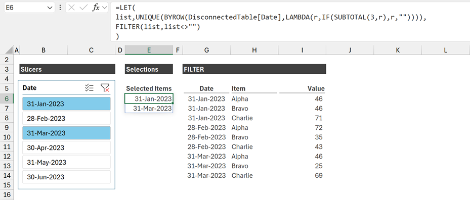
Let’s see how we can get the list of slicer selections from the Date column of the Data table.

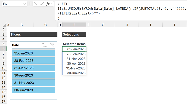
The formula in cell E6 is:

=LET(
list,UNIQUE(BYROW(Data[Date],LAMBDA(r,IF(SUBTOTAL(3,r),r,"")))),
FILTER(list,list<>"")
)

This is quite complex, so let’s break down this formula to understand what it does.

SUBTOTAL(3,r)

• 3 tells SUBTOTAL to perform a COUNTA operation (it counts numbers, text and boolean).
  • Rows that are visible, calculate as 1
  • Rows that are hidden by the filter, calculate as 0
• r is a placeholder to represent each row in a range. We will see more of r in the coming sections.

Next, let’s consider the IF function.

IF(SUBTOTAL(3,r),r,"")

In our scenario, SUBTOTAL will be calculated on each cell in a column.

• If the row is visible, SUBTOTAL returns 1 (which is equal to TRUE). Therefore, IF returns r (the cell value).
• If the row is hidden, SUBTOTAL returns 0 (which is equal to FALSE). Therefore, IF returns a blank text string ( “” ).

The next section is a BYROW/LAMBDA combination:

BYROW(Data[Date],LAMBDA(r,IF(SUBTOTAL(3,r),r,"")))

The BYROW/LAMBDA combination performs a calculation for each cell in the Data[Date] column.

As it calculates, each cell in that column is represented by r. And, each r is which is passed into the IF/SUBTOTAL functions.

It starts with the first cell in the Data[Date] column which has a value of 31-Jan-2023. If the row is visible the formula above returns 31-Jan-2023, if not it returns “”.

This continues for each row, and the results are joined together to return a list of values.

This result could contain duplicate values; we need to remove these.

UNIQUE(BYROW(Data[Date],LAMBDA(r,IF(SUBTOTAL(3,r),r,""))))

UNIQUE returns one instance of each visible value.

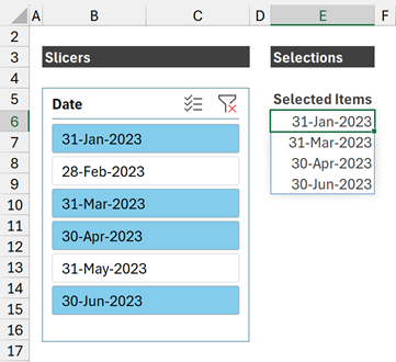
Assuming 31-Jan-2023 and 31-Mar-2023 are selected, the value returned by UNIQUE will be {31-Jan-2023;””;31-Mar-2023}.

Finally, lets remove the blank text string. We use the FILTER function for this.

=LET(
list,UNIQUE(BYROW(Data[Date],LAMBDA(r,IF(SUBTOTAL(3,r),r,"")))),
FILTER(list,list<>"")
)

We don’t want to include the UNIQUE/BYROW/LAMBDA/IF/SUBTOTAL combination twice. For efficiency we use LET to create a variable called list. Then, we use FILTER to remove any empty text strings from list.

The result of this formula is a list of the items selected by the slicer.

Changing and applying table slicer selections

Now we have the list of selected values, we can use them as we wish. Let’s suggest we want to include the value to date based on the maximum date selected.

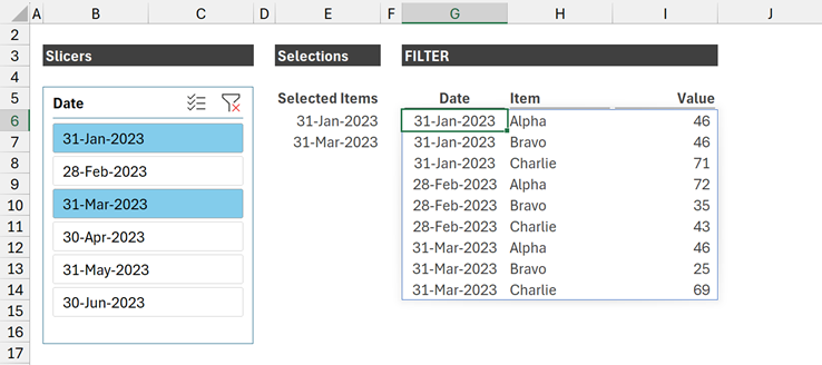
The formula in cell G6 is:

=FILTER(Data,Data[Date]<=MAX(E6#))

Even though 31-Jan-2023 and 31-Mar-2023 are selected; the formula returns all values which are less than or equal to 31-Mar-2023.

If we had multiple years in our data, we could calculate year-to-date as follows:

=FILTER(Data,(Data[Date]<=MAX(E6#))*(Data[Date]>=DATE(YEAR(MAX(E6#)),1,1)))

As you can imagine, there are almost an infinite number of scenarios we could use here.

Disconnected slicers

If we have multiple slicers connected to the same Table, they all influence each other. For complete freedom, we can use separate Tables with a slicer attached to each.

In the example file, we also have a separate Table called DisconnectedTable that only includes a Date column.

We created a slicer for this Table and placed it on another sheet.

The formula in cell E6 is:

=LET(
list,UNIQUE(BYROW(DisconnectedTable[Date],LAMBDA(r,IF(SUBTOTAL(3,r),r,"")))),
FILTER(list,list<>"")
)

This is exactly the same formula as before, but it references the DisconnectedTable[Date] column.

For the FILTER in G6 we can use exactly the same function as created in the section above.

The formula in G6 remains as:

=FILTER(Data,Data[Date]<=MAX(E6#))

If we want to include the items selected in the slicer, we would use the method from this post: How to FILTER by a list in Excel (including multiple lists). For that scenario, the formula would be:

=FILTER(Data,COUNTIFS(E6#,Data[Date]))

We can use the slicer values to control almost any formula. Hopefully, you can see how flexible this approach is.

Slicer selections LAMBDA

To make this easier to apply, we can create a reusable function.

Copy the following into a named range, and call it fxSlicerSelection

=LAMBDA(tableColumn,LET(list,UNIQUE(BYROW(tableColumn,LAMBDA(r,IF(SUBTOTAL(3,r),r,"")))),FILTER(list,list<>"")))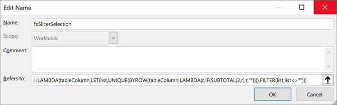

Now we can use fxSlicerSelection as a standard formula.

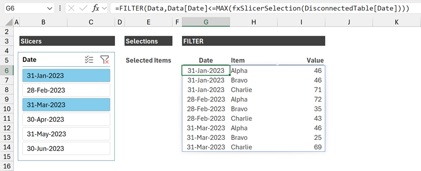
The formula in cell G6 is:

=FILTER(Data,Data[Date]<=MAX(fxSlicerSelection(DisconnectedTable[Date])))

We have used our custom fxSlicerSelection function directly in the FILTER function.

Conclusion

In this post, we have gone deep into Table slicers. We have seen how to:

• Get slicer selections as a list – extract the selected items
• Change filter context – adjust a user’s slicer selections
• Create disconnected slicer tables – separate tables that exist purely for creating slicers
• Build a reusable LAMBDA function – removes the need to write a complex formula each time we want to use this technique

In this post, we have only used the FILTER function, but we could use these in any dynamic array formula.

Related Posts

• How to use slicers with PIVOTBY, GROUPBY & FILTER in Excel
• Using Slicers with dynamic array formulas in Excel
• How to make cross filter visuals in Excel (amazing interactive visuals)

---

What next?

Discover how you can automate your work with our Excel courses and tools.