Using Slicers with dynamic array formulas in Excel

A few years back, I created a YouTube video about using slicers with formulas in Excel. It was a pretty popular video. That method used a dummy PivotTable, to act as the criteria for the formulas to calculate on. Today, I want to bring you a cleaner option for using slicers with formulas. This method uses only an Excel Table and dynamic array functions.

Slicers are an excellent tool for adding interactivity. When a user clicks on a slicer button, the results change to include only those selected items. Slicers are compatible with PivotTables, PivotCharts, Cube formulas, and Tables…but not standard formulas. So, let’s see how we can use a Table in a new way to get around this limitation.

This approach is deceptively simple. But like most things in Excel, the skill is knowing how to connect features together.

Table of Contents

• The example data
• Visible row functions
• Create the Slicer
• Connecting the Slicer to the formula
• Using a LAMBDA (advanced)
• Conclusion

Watch the video

Watch the video on YouTube.

The example data

The data used in the example is as follows:

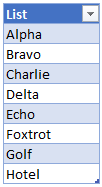
This is a Table called List, with a single column, also called List.

Visible row functions

In Excel, there are special functions that only calculate on visible rows. I believe there are only two SUBTOTAL and AGGREGATE.

We will not go into SUBTOTAL or AGGREGATE in detail in this post. But if you want to know more, here are some useful references:

• SUBTOTAL – https://exceljet.net/excel-functions/excel-subtotal-function
• AGGREGATE – https://exceloffthegrid.com/aggregate-the-best-excel-function-youre-not-using/

For our example, we will use the SUBTOTAL function.

The screenshot below shows a Table with the COUNTA, visible cells only, version of the SUBTOTAL function at the bottom. The total counts the number of visible rows. If we filter the Table, the total changes. Notice that the total at the bottom changes from 8 when unfiltered, to 3 when we have selected 3 items.

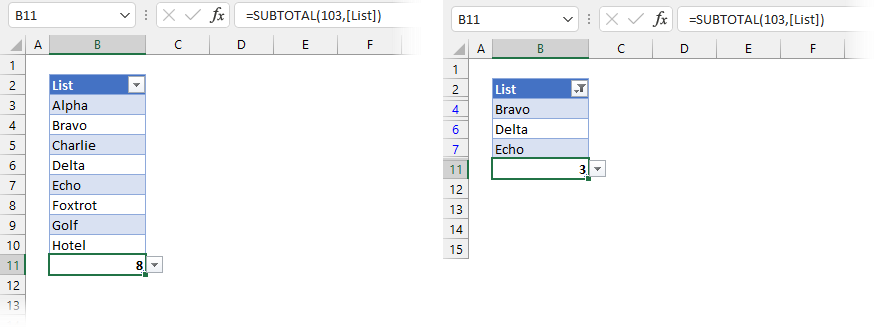
The formula in Cell B11 is:

=SUBTOTAL(103,[List])

The first argument of 103 tells SUBTOTAL to count cells while ignoring hidden rows; [List] is the Table name.

Instead of using SUBTOTAL for the total, let’s add a column called Include and use SUBTOTAL on each line. This method returns 1 for each visible row, or 0 for a hidden row. Of course, we can’t see the hidden rows, so we can’t see the result of the formula, but the hidden rows are 0 (I promise).

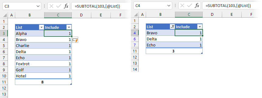
The formula in Cell C3 is:

=SUBTOTAL(103,[@List])

As we are using an Excel Table, the formulas copy down into each row automatically

Create the Slicer

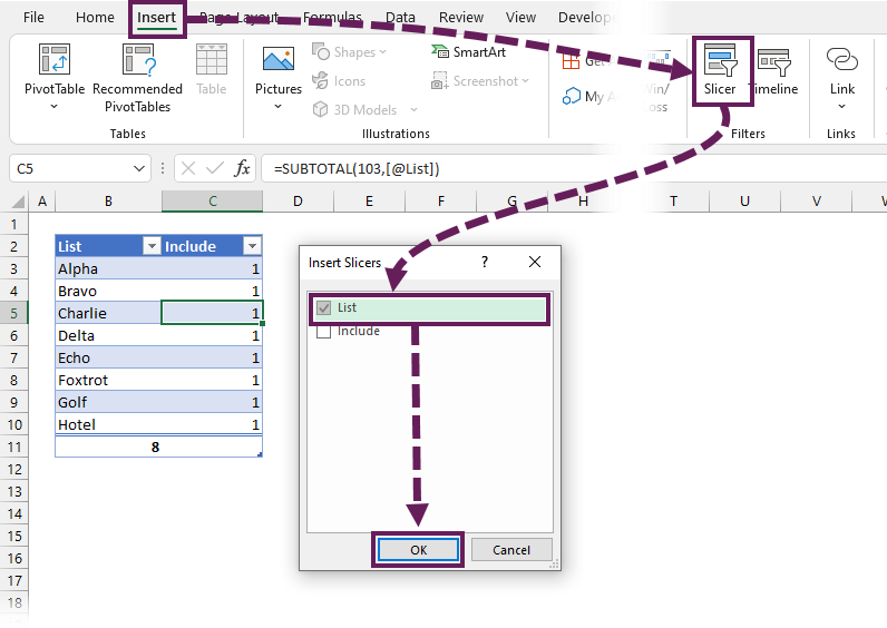
Let’s create the Slicer to use with our data.

1. Select a cell inside the Table
2. Click Insert > Slicer from the ribbon
3. The Insert Slicers dialog box will open
4. Check the required column
5. Click OK
   

Clicking the Slicer will filter the Table.

Connecting the Slicer to the formula

The next step is to get the plumbing to work between the Table and a formula.

We will use the FILTER function to return only the visible rows from the Table, which is only those with 1 in the Include column.

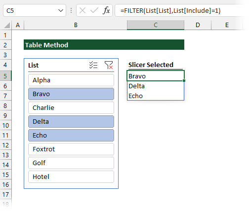
The formula in Cell C5 is:

=FILTER(List[List],List[Include]=1)

This formula returns an array of all items in the List column where the corresponding value in the Include column is equal to 1 (i.e., only the visible rows).

To learn more about the FILTER function, check out this post: FILTER function in Excel

Now, start clicking on the Slicer; as the selection changes, so does the returned array.

Using a LAMBDA (advanced)

Are you thinking: “Do we really need to use that extra column in the Table? Can’t we just create one formula to handle this?”.

The answer is, Yes, we can.

Notes:

• I must give thanks to Sergei Baklan for helping with this formula. I created something that worked but was hideous to read. Sergei was able to create a much nicer function; therefore, I have used Sergei’s formula below.
• At the time of writing, this solution uses functions only available on the Beta channel. Therefore, this may not work on your version of Excel.

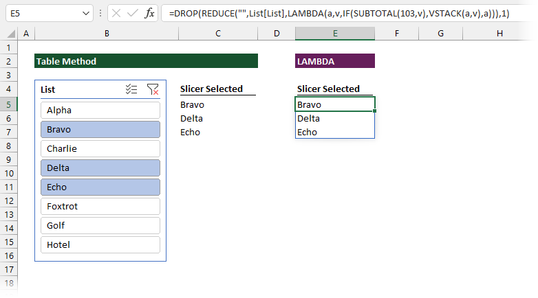
The formula in Cell E5 is:

=DROP(REDUCE("",List[List],LAMBDA(a,v,IF(SUBTOTAL(103,v),VSTACK(a,v),a))),1)

This post isn’t about LAMBDA functions, so we won’t go through the formula line by line. Effectively the formula applies the SUBTOTAL to each row in the Table. All the rows which return 1 (i.e., those which are visible) are stacked into a single array, and returned to the worksheet.

To use for your scenario, just replace List[List] with the Table and column name you are using. The remainder of the function will just do its thing and spill the required results.

Conclusion

Excel does not give us a simple way to use Slicers with formulas. With this approach, we can extract the selections with a dynamic array function, and then use those values to drive other calculations.

Check out my previous YouTube video for other formula techniques that can be used with this approach.

---

What next?

Discover how you can automate your work with our Excel courses and tools.