How to use slicers with PIVOTBY, GROUPBY & FILTER in Excel

Microsoft recently announced the GROUPBY and PIVOTBY functions for Excel. Because these new functions provide PivotTable-type functionality, many have asked if we can use slicers with these functions.

The answer is Yes!

So, in this post, we look at how to use slicers with PIVOTBY in Excel. But, we also go one step further and apply the same approach to the FILTER function too.

Notes:

• At the time of writing, GROUPBY and PIVOTBY are only available to those on the Microsoft 365 beta channel.

Table of Contents

• Data
• How to insert a slicer
• PIVOTBY function
• Connecting the slicer
• BYROW/LAMBDA/SUBTOTAL combination
• How does BYROW/LAMBDA/SUBTOTAL work?
• FILTER Function
• What about new data?
• Conclusion

Watch the video

Watch the video on YouTube

Data

The example data is in a Table called Data.

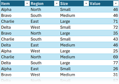
For this method to work, the slicer must be created from the same Table as the one used for the PIVOTBY function. An alternative method works with disconnected Tables; we are not covering that in this post.

How to insert a slicer

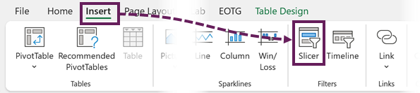
To insert a slicer, select a cell in the Table, then click Insert > Slicer.

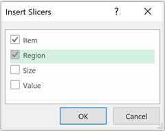
The Insert Slicers dialog box appears. Select the required slicers, then click OK. To work along with the example, insert slicers for both Item and Region.

Clicking the slicer buttons filters the Table, leaving the selected rows visible and the other rows hidden.

Cut and paste the slicers onto the required sheet.

PIVOTBY function

Let’s create our PIVOTBY function.

This post is not specifically about PIVOTBY, so if you want to know more about PIVOTBY, check out this post: New aggregation functions: GROUPBY and PIVOTBY

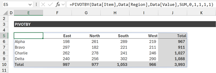
The formula in cell E5 is:

=PIVOTBY(Data[Item],Data[Region],Data[Value],SUM,0,1,1,1,1)

The arguments in order are:

• Data[Item] – row_fields: The values to display in the rows.
• Data[Region] – column_fields: The values to display in the columns.
• Data[Value] – values: The values to perform the calculation on.
• SUM – function: The calculation to perform on the values argument.
• 0 – field_headers: The data range does not include the column headers.
• 1 – total_row_depth: Show grand totals for rows.
• 1 – row_sort_order: Rows sorted by the first column in ascending order.
• 1 – total_col_depth: Show grand totals for columns.
• 1 – col_sort_order: Columns sorted by the first row in ascending order.

Connecting the slicer

The remaining argument of PIVOTBY, which we have not used yet, is filter_array. This argument determines which values are included/excluded in the calculation.

We need to create a calculation that returns TRUE/FALSE for each row in the source Table.

• TRUE or 1: The row is included in the PIVOTBY calculation
• FALSE or 0: The row is excluded from the PIVOTBY calculation

BYROW/LAMBDA/SUBTOTAL combination

To calculate 1 or 0, we can use the SUBTOTAL function (AGGREGATE is an alternative).

SUBTOTAL calculates values based on visible cells. So, if we use the COUNTA version of SUBTOTAL on each row, it returns:

• 1 if the row is visible
• 0 if the row is hidden

With this knowledge, let’s update PIVOTBY to include the filter_array argument.

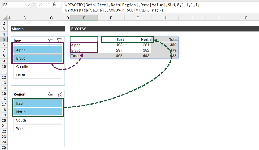
The formula in cell E5 is:

=PIVOTBY(Data[Item],Data[Region],Data[Value],SUM,0,1,1,1,1,
BYROW(Data[Value],LAMBDA(r,SUBTOTAL(3,r))))

If we select buttons in either the Item or Region slicer, the PIVOTBY updates.

How does BYROW/LAMBDA/SUBTOTAL work?

Let’s break down this function to try and understand each part.

SUBTOTAL is an aggregation function that returns a single value. However, we need to return a separate value for each row of the source Table. Therefore, we use BYROW & LAMBDA to perform the SUBTOTAL calculation once on each row.

SUBTOTAL(3,r)

• 3 tells the SUBTOTAL function to perform a COUNTA operation (counts numbers, text, and boolean).
  • Visible rows calculate as 1
  • Rows hidden by the filter calculate as 0
• r is a placeholder to represent the value from a row.

The next section is the BYROW/LAMBDA combination:

LAMBDA(r,SUBTOTAL(3,r))

LAMBDA creates a reusable function. This means we can calculate SUBTOTAL over-and-over to return a value for each item in r.

BYROW(Data[Item],LAMBDA(r,SUBTOTAL(3,r)))

BYROW tells the LAMBDA function which items to calculate over, in the formula above it is performed for each row in the Data[Item] column. Each row of the Data[Item] column is treated as r.

To apply this combination to your scenario, you only need to change Data[Item] to the name of a column in your data.

FILTER Function

filter_array has the same syntax as the include argument of the FILTER function. Therefore, we can use the same BYROW/LAMBDA/SUBTOTAL combination inside FILTER.

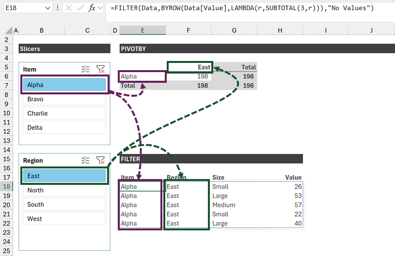
The formula in cell E18 is:

=FILTER(Data,BYROW(Data[Value],LAMBDA(r,SUBTOTAL(3,r))),"No Values")

Using the same BYROW/LAMBDA/SUBTOTAL calculation, FILTER also responds to slicer selections.

The final result is that we have PIVOTBY that simulates a PivotTable and FILTER that gives us the breakdown of the value.

Find out more about FILTER here: FILTER function in Excel.

What about new data?

In our example, the formulas are based on a single Table. Therefore, when we add new data to the Table, the slicer buttons and the formulas update to include that data automatically.

Conclusion

In this post, we have seen how to use slicers with the PIVOTBY and FILTER functions. GROUPBY behaves in exactly the same way.

The key is the BYROW/LAMBDA/SUBTOTAL combination, which returns a 1 or 0 value for each row in the Table.

So, now you know. YES, we can use slicers with PIVOTBY, GROUPBY, and FILTER in Excel.

Related Posts:

• How to FILTER by a list in Excel (including multiple lists)
• Using Slicers with dynamic array formulas in Excel
• FILTER function in Excel (How to + 8 Examples)

---

What next?

Discover how you can automate your work with our Excel courses and tools.