How to use SUMIFS with arrays (Excel problem solved!)

Over the past months, the topic of using SUMIFS with arrays has come up a few times, so I thought I would write a post to help anyone with the same question.

While I’m using SUMIFS throughout this post, it equally applies to SUMIF, COUNTIF, COUNTIFS, MAXIF, MAXIFS, MINIF, MINIFS, AVERAGEIF, and AVERAGEIFS.

Table of Contents

• Example
• The problem with the SUMIFS function
• Using range functions to solve the problem
• Using FILTER to solve the problem
• How to simulate spilling with SUMIFS
• GROUPBY – the ultimate solution?
• Conclusion – SUMIFS with arrays

Watch the video

Watch on YouTube

Example

Let’s start by looking at an example.

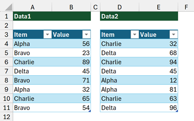
In the example workbook, we have two Tables: Data1 and Data2. We want to calculate the total of an Item from the combined tables.

We will break down the formula into stages to make it easier to explain.

We start by stacking the Tables into an array using VSTACK.

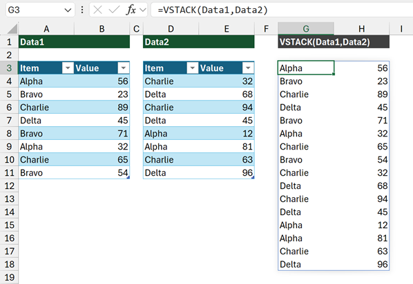
Cell G3 contains a formula to stack the tables vertically:

=VSTACK(Data1,Data2)

The values start at G3 and spill into the remaining rows. So far, so good, no issues.

Now let’s perform the SUMIFS:

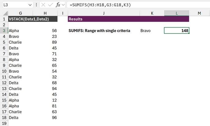
The formula in cell L3 is:

=SUMIFS(H3:H18,G3:G18,K3)

This sums the cells from H3:H18 where the equivalent cells in G3:G18 are equal to K3 (Bravo).

This works, but it is not dynamic. If we add new rows to Data2, the VSTACK function includes the new row, but the formula ranges for SUMIFS do not expand.

So, let’s change up our formula to include CHOOSECOLS. This function allows us to choose a column from an array.

=SUMIFS(CHOOSECOLS(G3#,2),CHOOSECOLS(G3#,1),K5)

• G3# – The spill range created by the VSTACK function.
• CHOOSECOLS(G3#,2) – selects the values in the 2nd column of the spill range.
• CHOOSECOLS(G3#,1) – selects the values in the 1st column of the spill range.

We now have exactly the same values, in exactly the same positions within SUMIFS. So, this should work… right?

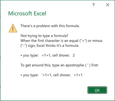
…unfortunately, this causes an error.

The error message is not particularly helpful, as it doesn’t really tell us what the problem is.

The problem with the SUMIFS function

Before dynamic arrays, we used SUMIFS, and all the other xxxxIF and xxxxIFS functions quite happily. So, what’s the issue?

If we look at the syntax of SUMIFS, the issue becomes clear.

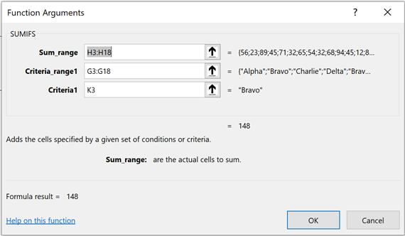
The arguments refer to ranges: sum_range, criteria_range1, etc. Even the description of sum_range is “actual cells to sum”.

So, we can see from this that SUMIFS works with ranges, but not with arrays. That is the problem.

But, don’t worry we have lots of alternatives.

Using range functions to solve the problem

In Excel, there are special formulas that return ranges. Since G3# is a range reference, we could use one of those range functions inside SUMIFS.

One of the range functions is INDEX.

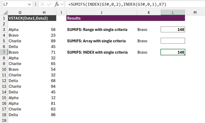
The formula in cell L7 is:

=SUMIFS(INDEX(G3#,0,2),INDEX(G3#,0,1),K7)

• INDEX(G3#,0,2) – Returns the range of cells from the G3# spill range.
  • 0 = all rows
  • 2 = second column
• INDEX(G3#,0,1) – Returns the range of cells from the G3# spill range.
  • 0 = all rows
  • 2 = second column

This is very similar to CHOOSECOLS. However, CHOOSECOLS returns an array, while in this context, INDEX returns a range.

Therefore, SUMIFS accepts the output of INDEX as a range for the sum_range and criteria_range1 arguments. The results are calculated correctly.

This is where things get a little confusing.

If we replace G3# (a range reference) with an array (VSTACK(Data1,Data2)), this passes an array into sum_range and criteria_range1 and causes an error.

For example, the following formula will not work.

=SUMIFS(INDEX(VSTACK(Data1,Data2),0,2),INDEX(VSTACK(Data1,Data2),0,1),K7)

This demonstrates that it’s not INDEX by itself but how we use INDEX that matters.

Using FILTER to solve the problem

We’ve seen we can only use SUMIFS where a range is passed into the function. However, there are alternative solutions that use arrays.

First, let’s FILTER to the values we wish to calculate:

=FILTER(CHOOSECOLS(G3#,2),CHOOSECOLS(G3#,1)=K9)

The above formula returns an array of values for the rows matching with Bravo: {23;71;54}

Now let’s wrap FILTER in the SUM function:

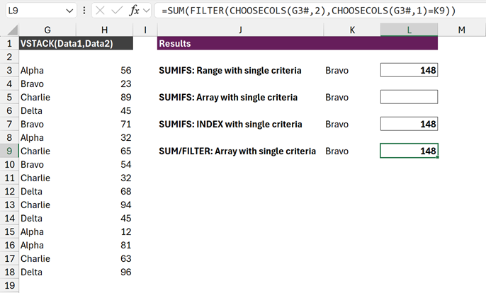
The formula in cell L9 is:

=SUM(FILTER(CHOOSECOLS(G3#,2),CHOOSECOLS(G3#,1)=K9)

This shows that we can use FILTER to return matching values, then SUM the result to achieve the same result as SUMIFS.

Because all the formulas involved handle arrays, we can use VSTACK directly in the formula without needing to reference the G3# spill range.

=SUM(FILTER(CHOOSECOLS(VSTACK(Data1,Data2),2),CHOOSECOLS(VSTACK(Data1,Data2),1)=K9))

How to simulate spilling with SUMIFS

You might be thinking… “Yes, but SUMIFS spills when we provide multiple criteria. How can we achieve that?“

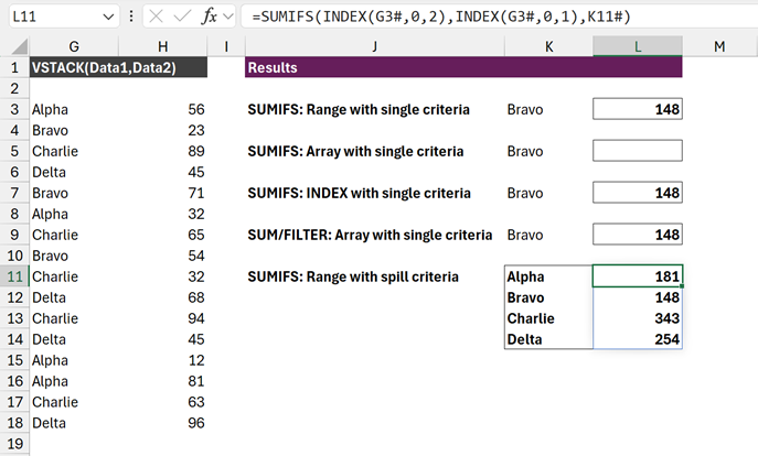
The formula in cell K11 creates a unique list of items.

=SORT(UNIQUE(CHOOSECOLS(G3#,1)))

So, if we use a range function (INDEX, for example), we can spill the results and maintain the dynamic range.

The formula in cell N11 calculates a result for all the items in the spill range K11#.

=SUMIFS(INDEX(G3#,0,2),INDEX(G3#,0,1),K11#)

If we want to spill in the same way using the FILTER function, we must revert to another method.

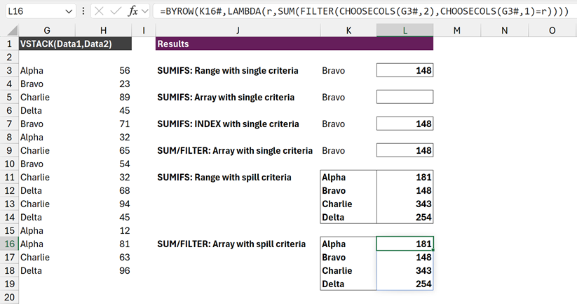
The formula in cell L16 is:

=BYROW(K16#,LAMBDA(r,SUM(FILTER(CHOOSECOLS(G3#,2),CHOOSECOLS(G3#,1)=r))))

Please check out this post for full details of how this works: How to spill multiple FILTER functions in Excel.

GROUPBY – the ultimate solution?

Microsoft recently announced the GROUPBY function in Excel (at the time of writing it is only available to those on the Microsoft 365 Beta channel).

GROUPBY gives us a new way to perform calculations based on grouping. Ultimately, summing by a criteria and summing a group provides the same result. Therefore, we could use GROUPBY as an alternative to SUMIFS.

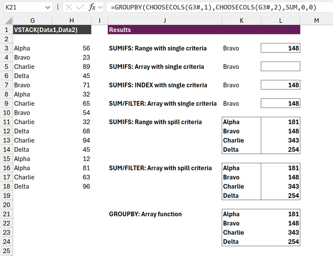
The formula in cell K21 is:

=GROUPBY(CHOOSECOLS(G3#,1),CHOOSECOLS(G3#,2),SUM,0,0)

This formula spills the categories and SUM result for all the values, without any header row and without any total).

So, this gives us the same result as SUMIFS.

Conclusion – SUMIFS with arrays

The xxxxIF and xxxxIFS functions in Excel are built to work with ranges and not arrays.

So, if we want to use arrays, we must use other formula techniques. The SUM/FILTER combination or GROUPBY both provide a good basis for performing array calculations equivalent to SUMIFS.

Related posts:

• How to spill multiple FILTER functions in Excel
• How to FILTER by a list in Excel (including multiple lists)
• FILTER function in Excel (How to + 8 Examples)

---

What next?

Discover how you can automate your work with our Excel courses and tools.