Calculate quarter from dates in Excel (inc non-standard calendars)

In many companies, analyzing by quarter is common practice. Unfortunately, when we calculate quarter from dates in Excel, we can make things overly complex. This is especially true when working with financial years that do not align with the calendar year. Or even worse, non-standard calendars (such as 4-5-4 or 4-4-5)!

So, in this post, we explore how to calculate quarter from dates in all scenarios.

Table of Contents

Standard calendar year
Financial year not aligned to calendar year
Non-standard calendar
Conclusion

Download the example file: Click the button below to join the Insiders program and gain access to the example file used for this post.

File name: 0191 Quarter from dates.zip

Get access

Watch the video

Calculate quarter from dates in Excel | Calendar Year, Financial Year, Non-Standard Calendars

Watch on YouTube

Standard calendar year

Calculating a quarter from a date is reasonably straightforward when working with calendar years. We can use a combination of the MONTH and ROUNDUP functions.

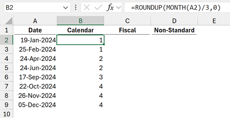
Quarter from dates in Excel - Calendar month

The formula in cell B2 is:

=ROUNDUP(MONTH(A2)/3,0)

Let’s break down this formula to understand what’s happening.

=ROUNDUP(MONTH(A2)/3,0)

MONTH(A2) calculates the month (i.e., a value from 1 to 12).

Using 19-Jan-2024 as an example – this calculates to 1, as January is the first month.

=ROUNDUP(MONTH(A2)/3,0)

In the next step, we divide the result from MONTH(A2) by 3. This is because there are 3 months in a quarter.

Continuing with our example: 1/3 = 0.33333

=ROUNDUP(MONTH(A2)/3,0)

Finally, we take the result from the previous step and round up to the next whole number.

In our example, 0.33333 rounds up to 1.

Therefore, 19-Jan-2024 is in quarter 1.

If we want to prefix the letter Q, we can easily add that to the formula.

="Q"&ROUNDUP(MONTH(A2)/3,0)

The remaining examples in this post follow a similar structure. The only element that changes is how we calculate the month number.

Financial year not aligned to calendar year

Things become a little trickier when the financial year does not align with the calendar year. But don’t worry; we’ve got this 👍.

For our example, let’s assume that the year-end is 31 August. Therefore, the quarters are

Q1 – Sep, Oct, Nov
Q2 – Dec, Jan, Feb
Q3 – Mar, Apr, May
Q4 – Jun, Jul, Aug

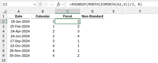
Quarter from dates in Excel - Fiscal month

The formula in cell C2 is:

=ROUNDUP(MONTH(EOMONTH(A2,4))/3, 0)

Let’s break down this formula.

=ROUNDUP(MONTH(EOMONTH(A2,4))/3, 0)

EOMONTH(A2,4) adjusts a date to be the month-end, 4 months in the future.

The value is 4 because if August is the year-end, it is the 12th month. Since August is the 8th month of the calendar year, we adjust by 4 to get to the 12th month.

In our example, 19-Jan-2024, the end of the month 4 months in the future is 31 May 2024.

=ROUNDUP(MONTH(EOMONTH(A2,4))/3, 0)

Next, we extract the MONTH from 31 May 2024, which is 5.

=ROUNDUP(MONTH(EOMONTH(A2,4))/3, 0)

Finally, we divide by 3 and round up to get the quarter number. Which, for our example date, is 2.

Non-standard calendar

Now for the worst option… the non-standard calendar. These are commonly known as 4-4-5 or 4-5-4 calendars.

These non-standard calendars have exactly 52 weeks. Therefore, every few years, to re-align the year-end, there is a 53-week year, which might create a 4-5-5 or a 4-4-6 calendar.

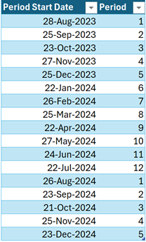
As a result, we cannot guarantee when the end of a period will be. So, we need to start by creating a calendar Table.

Let’s assume we have a 4-4-5 calendar table called Dates. The year starts on 28-Aug-2023.

Now let’s use this table in a formula.

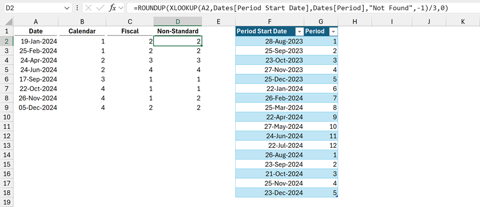
Quarter from dates in Excel - Non-standard calendar

The formula in cell D2 is:

=ROUNDUP(XLOOKUP(A2,Dates[Period Start Date],Dates[Period],"Not Found",-1)/3,0)

Let’s look at the XLOOKUP section in more detail.

=ROUNDUP(XLOOKUP(A2,Dates[Period Start Date],Dates[Period],"Not Found",-1)/3,0)

In this formula, XLOOKUP is:

A2: The value to lookup.
Dates[Period Start Date]: The column to look up in.
Dates[Period]: The column to return a value from.
“Not Found”: The value to return if the lookup value does not exist in the table.
–1: Return the exact match or next smallest item.

Using 19-Jan-2024 as our example – XLOOKUP matches against 21-Jan-2024 (i.e., the next smallest item) and returns the corresponding value from the Period column, which is 5.

=ROUNDUP(XLOOKUP(A2,Dates[Period Start Date],Dates[Period],"Not Found",-1)/3,0)

Finally, we divide by 3 and round up to get the quarter number. For our example, the quarter is 2.

See, even with non-standard calendars, it’s not so bad. 😁

NOTE:

We are not restricted to XLOOKUP (available in Excel 2021 and Excel 365). We could also use:

INDEX/MATCH

=ROUNDUP(INDEX(Dates[Period],MATCH(A2,Dates[Period Start Date]))/3,0)

or VLOOKUP

=ROUNDUP(VLOOKUP(A2,Dates,2)/3,0)

Conclusion

Calculating quarters from a date in Excel is a common task, especially when dealing with financial data.

Thankfully, it doesn’t matter if we are working with a calendar year, financial year, or a non-standard calendar. Excel can handle it. We just need to adjust the month calculation to match the scenario.

Related posts:

What next?

Discover how you can automate your work with our Excel courses and tools.