How to spill multiple FILTER functions in Excel

In a recent project, I used FILTER and TEXTJOIN to create a comma-separated list to display in a cell. Unfortunately, when I tried to spill the values for different filter criteria, it created an error. So, in this post, we will work through a solution, showing how to spill multiple FILTER functions in Excel.

Watch the video

Watch the video on YouTube

Example

In the example workbook, there are two Tables: POs (Purchase Orders) and Invoices:

Table: POs

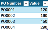
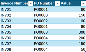
Table: Invoices

From these Tables, there is a summary showing the PO value, Invoice value, and Variance for each PO.

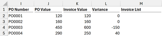
Cell I2 contains a dynamic array formula to display the PO Numbers from the POs Table in alphabetical order.

=SORT(UNIQUE(POs[PO Number]))

=SORT(UNIQUE(VSTACK(POs[PO Number],Invoices[PO Number])))

Cell J2 contains a formula to display the total value for each PO.

=SUMIFS(POs[Value],POs[PO Number],I2#)

Cell K2 contains a formula to display the amount invoiced per PO.

=SUMIFS(Invoices[Value],Invoices[PO Number],I2#)

Finally, cell L2 calculates the variance between the PO Value and Invoice Value.

=J2#-K2#

These are dynamic array formulas; if new purchase order numbers are added to the POs table, the report updates automatically.

The goal is to list the invoice numbers relating to the PO, as shown in cell M2 below.

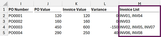
It should be pretty easy… right?… or maybe not.

Single FILTER function

Let’s start by building a FILTER function:

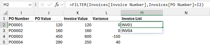
Cell M2 contains the following formula:

=FILTER(Invoices[Invoice Number],Invoices[PO Number]=I2)

The spill range returned by the FILTER contains the two invoice numbers that match PO0001.

Now, let’s wrap FILTER in a TEXTJOIN to get a comma-separated list of invoices in a single cell.

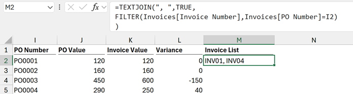
The formula in cell M2 is:

=TEXTJOIN(", ",TRUE,
FILTER(Invoices[Invoice Number],Invoices[PO Number]=I2)
)

This gives us the invoices in a comma-separated list.

So far, so good.

The problem with multiple FILTER functions

So now, to get the FILTER to calculate for each PO Number, surely we only need to change I2 to I2# (the spill range of the PO numbers).

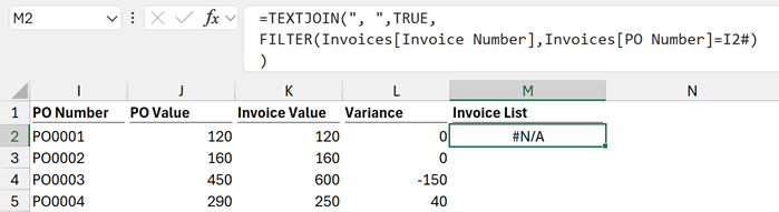
The formula in cell M2 is:

=TEXTJOIN(", ",TRUE,
FILTER(Invoices[Invoice Number],Invoices[PO Number]=I2#)
)

Unfortunately, that returns the N/A# error. That’s not what we want! 🤔

While FILTER is a dynamic array function that spills filter results, it cannot spill multiple FILTER calculations.

Multiple FILTER functions inside a Table

In our example, the TEXTJOIN/FILTER combination returns a single value. This means we can use it inside a Table without creating a #SPILL! error.

So, if we want to include the Invoice List inside the POs table, we simply include the TEXTJOIN/FILTER formula in the table column.

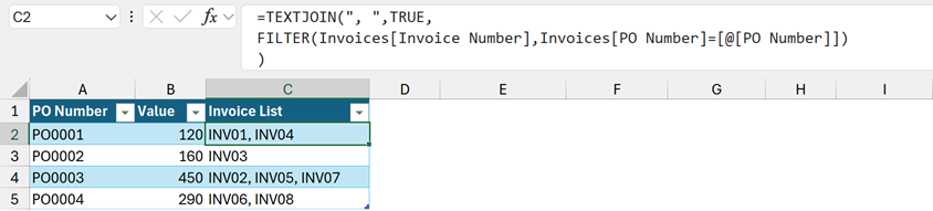
The formula in cell C2 is:

=TEXTJOIN(", ",TRUE,FILTER(Invoices[Invoice Number],Invoices[PO Number]=[@[PO Number]]))

The calculated column feature of Tables performs a separate calculation for each row. It is not a spill range.

Simple enough. So, if this works for Tables, how can we make this work for standard ranges?

BYROW & LAMBDA to spill multiple FILTER functions

Just as a table column performs individual calculations for each row, the BYROW/LAMBDA combination performs separate calculations for each row in an array.

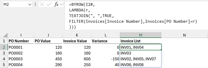
The formula in Cell M2 is:

=BYROW(I2#,
LAMBDA(r,
TEXTJOIN(", ",TRUE,
FILTER(Invoices[Invoice Number],Invoices[PO Number]=r)
)
))

This provides the result we want.

• LAMBDA takes variables and uses them in a function we define.
  In this scenario:
  • The variable is called r.
  • The TEXTJOIN/FILTER combination is the defined function.
  • r is used as the variable inside the TEXTJOIN/FILTER combination.
• BYROW tells LAMBDA to perform the calculation for each row in an array.
  In this scenario:
  • The array is the spill range of I2#
  • Each row in the array is passed into the LAMBDA to use as the r variable.

Alternative approach for stacking multiple FILTER functions

If you’re thinking: “But I haven’t aggregated FILTER down to a single value, this won’t work for me…”

There is an alternative DROP/REDUCE/LAMBDA/VSTACK approach we could use.

=DROP(
REDUCE(1,I2#,
LAMBDA(s,c,VSTACK(s,
TEXTJOIN(", ",TRUE,
FILTER(Invoices[Invoice Number],Invoices[PO Number]=c)
)
)))
,1)

This approach appends the result of each FILTER function using the VSTACK function; then it spills the final result.

This method works when FILTER returns multiple values, rather than a single value. This is more than we need for our example, but it may be what you need for your scenario.

Conclusion

In this example, we have seen:

• How to aggregate the values of a FILTER function into a string with TEXTJOIN.
• A calculated column performs a calculation for each row in the Table.
• Tables return dynamic arrays where the formula returns a single value.
• The BYROW/LAMBDA combination performs a calculation for each row of a spill range.

It just goes to prove, sometimes simple scenarios can be a little trickier than we might expect.

Related Posts:

• FILTER function in Excel (How to + 8 Examples)
• Dynamic arrays in Excel – Everything you NEED to know
• How to Find & Replace multiple words in Excel: REDUCE & SUBSTITUTE

What next?

Discover how you can automate your work with our Excel courses and tools.

Excel Academy
The complete program for saving time by automating Excel.

Find out more

Excel Automation Secrets
Discover the 7-step framework for automating Excel.

Find out more

Office Scripts: Automate Excel Everywhere
Start using Office Scripts and Power Automate to automate Excel in new ways.

Find out more