
As many regular readers will know, I’m a big fan of writing text dynamically. This means we don’t need to manually update text or headings in our reports. Instead, the text calculates and updates automatically. So, today I want to share how to Find and Replace multiple words in Excel using the REDUCE and SUBSTITUTE functions.
Let’s start by looking at the functions, then finding out how to use them together.
Table of Contents
Download the example file: Join the free Insiders Program and gain access to the example file used for this post.
File name: 0153 Find and replace multiple values.xlsx
Watch the video

SUBSTITUTE function in Excel
The SUBSTITUTE function finds and replaces text inside another value.
Syntax
=SUBSTITUTE(text, old_text, new_text, [instance])
- text: The text to change
- old_text: The text to find
- new_text: The text to replace with
- [instance]: The nth instance of the old_text to replace. This is an optional argument. If not supplied, all instances are replaced.
Example
Here is a simple example:
=SUBSTITUTE("Flori is my dog's name","dog","cat")Every instance of dog is replaced with cat.
Result: Flori is my cat’s name
NOTE: SUBSTITUTE is case-sensitive.
REDUCE function in Excel
The REDUCE function applies a LAMBDA function for each array element, returning the accumulated result.
In simple terms, REDUCE behaves like a looping function. It performs a calculation multiple times over an item and then returns a single final result. This might not sound useful, but by the end of this post, you will see its power.
Syntax
=REDUCE([initial_value], array, lambda)
- [initial_value]: The initial value of the accumulator. This is optional, as the initial value can be blank.
- array: The array for which a LAMBDA function is applied for each element
- lambda: The function to perform for each element
Find out more about REDUCE: https://exceljet.net/functions/reduce-function
LAMBDA
The last argument of REDUCE is lambda; this is the function to perform for each item in the array.
LAMBDA is a special type of function for making custom functions. When used with REDUCE, LAMBDA has a specific syntax we need to follow. Rather than risk confusing you any further, let’s look at an example so you can see how it works.
Find and Replace Multiple Words in Excel
OK, now it’s time to use these functions.
Example data
This is the example we are working with
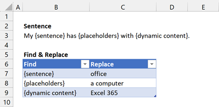
Cell B3 contains a template sentence. My {sentence} has {placeholders} with {dynamic content}.
Our goal is to find each word with curly brackets (e.g. {sentence}, {placeholders}, {dynamic content}) and replace it with a new word. The find and replace elements are contained in the Table called FindReplace (Cells B6:C9).
Apply the SUBSTITUTE function
Let’s start by applying the SUBSTITUTE function.
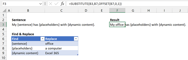
The formula in cell F3 is:
=SUBSTITUTE(B3,B7,OFFSET(B7,0,1))This is taking the value in B3, finding the value in B7, then replacing it with the value 1 column to the right of B7.
SUBSTITUTE can only include one find, and one replace value.
Using REDUCE with SUBSTITUTE
By using REDUCE, we can perform the SUBSTITUTE function for each item in the Find list.
Here is the final result:
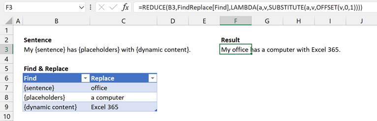
The formula in cell F3 is:
=REDUCE(B3,FindReplace[Find],LAMBDA(a,v,SUBSTITUTE(a,v,OFFSET(v,0,1))))
Let’s break this down:
- B3 is the initial value
- FindReplace[Find] is the list of items to find
- a: the parameter representing the SUBSTITUTE result at the end of each loop. It will start with the value in B3, but changes each time the calculation runs.
- v: the parameter representing each element in the FindReplace[Find] array.
The first time the calculation runs, SUBSTITUTE replaces {sentence} with office. This gives a result of My office has {placeholders} with {dynamic content}.
The second time the calculation runs, SUBSTITUTE replaces {placeholders} with a computer. This gives a result of My office has a computer with {dynamic content}.
The third time the calculation runs, SUBSTITUTE replaces {dynamic content} with Excel 365. This gives the final result of My office has a computer with Excel 365.
This shows that REDUCE has applied SUBSTITUTE for each item in the FindRepalce table.
Applying the formula to your scenario
The formula above may appear confusing. However, to apply it to your scenario, there are only 2 things you need to change.
=REDUCE(B3,FindReplace[Find],LAMBDA(a,v,SUBSTITUTE(a,v,OFFSET(v,0,1))))- B3: Change this to be your initial value
- FindReplace[Find]: Change this to be the values to find
Provided the Replace values are directly right of the Find values, the calculation will work for your scenario.
Conclusion
REDUCE and LAMBDA give us an excellent way of performing a calculation repeatedly.
Even if a function, like SUBSTITUTE, only performs a single action, wrapping it in REDUCE and LAMBDA causes that calculation to be undertaken multiple times.
Using the REDUCE and SUBSTITUTE combination, we can find and replace multiple words in Excel to calculate dynamic sentences and headings.
Related Posts:
- How to create dynamic text in Excel (TEXT + Number Formats)
- How to remove spaces in Excel (7 simple ways)
- Automatic commentary writing formula in Excel – Amazing LAMBDA
Discover how you can automate your work with our Excel courses and tools.
The Excel Academy

Make working late a thing of the past.
The Excel Academy is Excel training for professionals who want to save time.
How do you even think of these use cases?!
Brilliant!
I find a problem, I try to find the best way to solve it. Often it leads off on a tangent to look at things I’ve never thought of before.
Hi Mark,
Once again, a nicely explained function with unlimited potential. Imagine, if you will, using an xlookup formula to populate C7, C8, and C9. You could iterate through a long list of values making this even more valuable.
Regards,
Yes, you certainly could use XLOOKUP inside the REDUCE. I’m not sure it would give a better solution in the scenario. But now that you’ve mentioned it, I suspect there are other really good use cases… I might have to go and play.