How to combine rows in Power Query

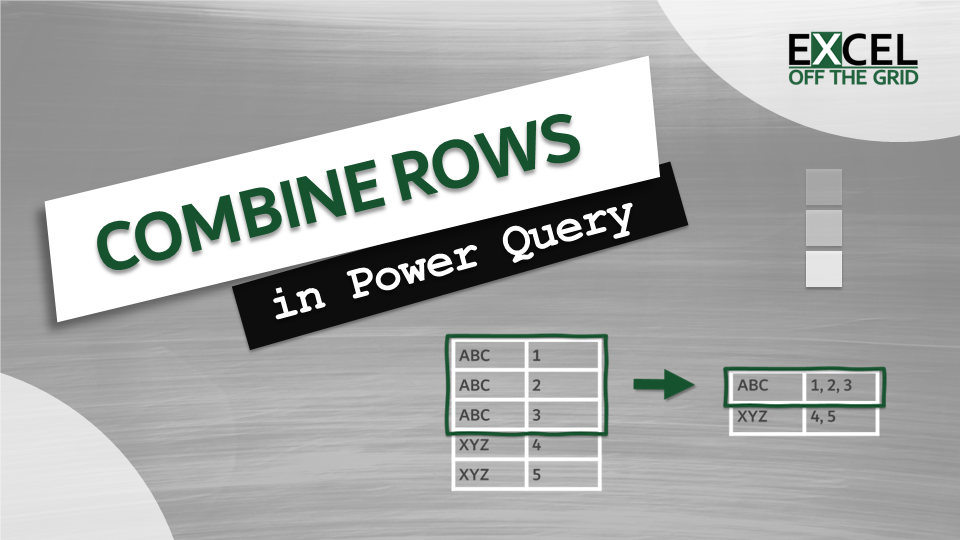
In this post, we look at how to combine rows with Power Query. The user interface gives us a way to merge columns, but there is no Power Query merge rows transformation. Therefore, I will show you how to achieve it in this post.

There are two common scenarios in which we need to merge rows:

• Merge all rows in the data set
• Merge specific rows (e.g., header rows)

Both are covered in this post.

Table of Contents

• Power Query combine rows across the entire dataset
• Scenario
• Load data into Power Query
• Merge columns
• Group by with Sum
• Editing the M Code
• Load data into Excel
• Power Query merge specific rows
• Scenario
• Convert the data into a Table
• Load the data into Power Query
• Data preparation
• Transpose, merge columns, transpose
• Load data into Excel
• Conclusion

Watch the video:

Watch the video on YouTube

Power Query combine rows across the entire dataset

While having a flat table is excellent for data manipulation, that may not always be optimal:

• It’s not how users wants to view the information
• May need to optimize for merging with other data sources

Therefore, even if we have a structured data layout, we may still need to combine rows.

Scenario

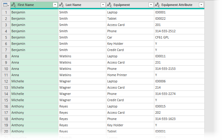
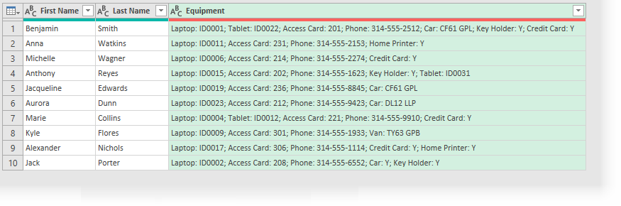
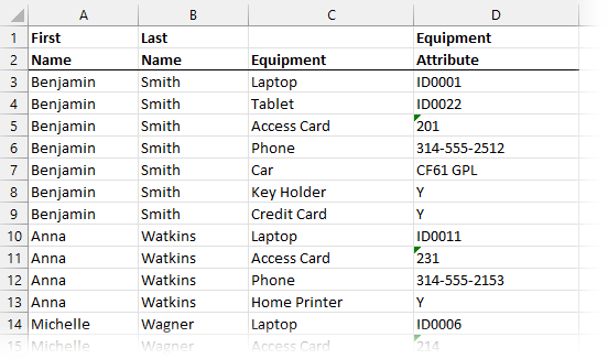
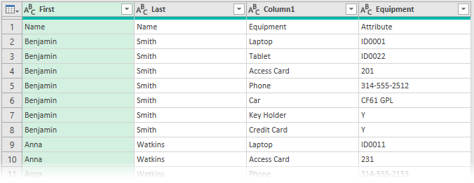
Here is the data from the example file:

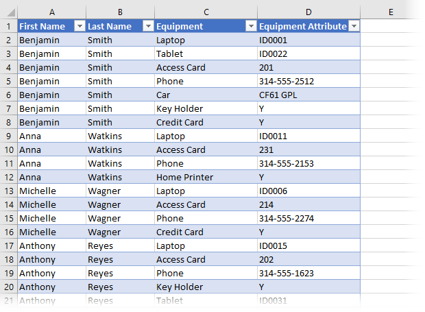
In the screenshot, we have a list of employees and any equipment the company has allocated to them. For example, we can see Anna Watkins has a laptop, access card, phone, and home printer.

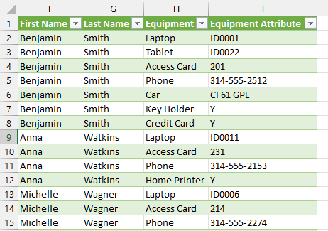
The goal is to combine all equipment information for each employee into a single cell (as shown below).

This all sounds simple, doesn’t it? Before Power Query, we would need to use complex formulas to achieve this result. But with Power Query, it becomes a few simple transformations.

OK, let’s get started.

Load data into Power Query

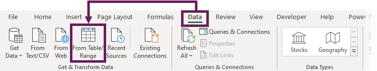
Select a cell within the data table, then click Data > From Table / Range.

The Power Query window opens and displays the data from the Table.

Now we’re ready to start the transformations.

Initially, we will combine Equipment and Equipment Attribute into a single column, then combine the rows into a single row for each employee.

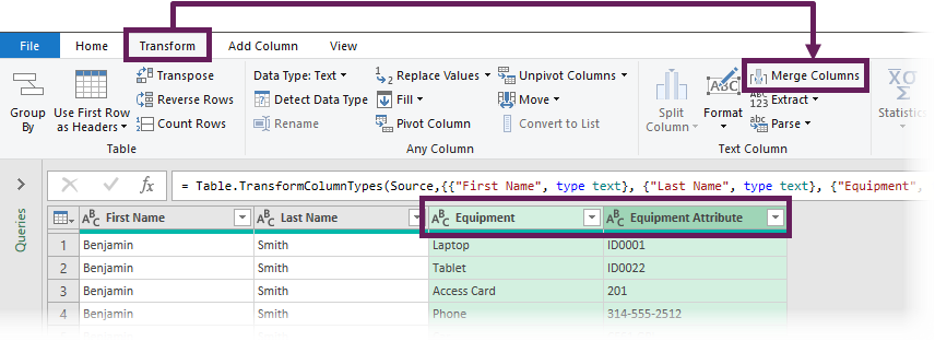
Merge columns

Select the Equipment and Equipment Attribute columns, then click Transform > Merge Columns

For our example, we want to place a colon and space between the two columns. So, we need to select –Custom– from the Separator drop-down list, and in the box below, enter Colon ( : ), followed by a space character.

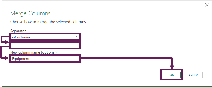
I’ve given the new column the name Equipment; then we can click OK.

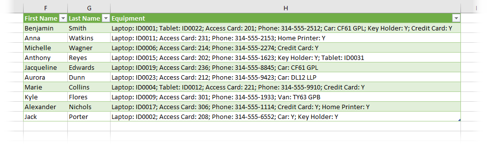
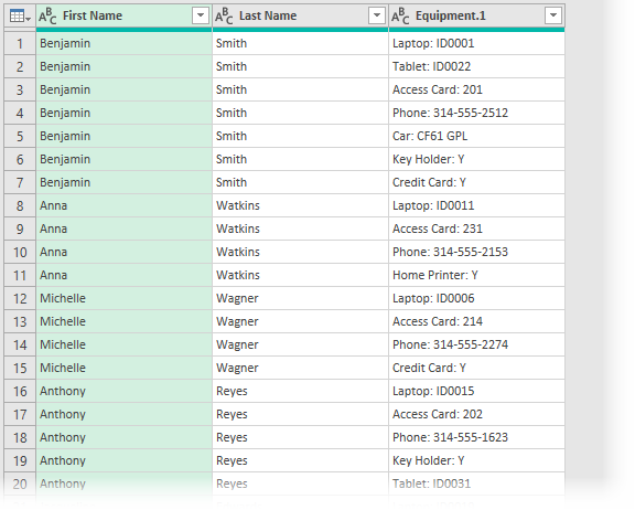
The Equipment and Equipment Attribute columns are combined into one, as shown by the screenshot below.

Group by with Sum

Now for the exciting part. In our next transformation, we create an error. But don’t worry, because I’ll explain why it occurs and what we do about it.

Select all the columns except the column to be combined. In our example, we need to select the First Name and Last Name columns.

Click Transform > Group By

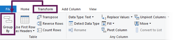
The Group By dialog box opens. The fields to complete are:

• New column name: Enter a name for the column of combined cells (I’ve used Equipment)
• Operation: Select Sum from the drop-down list
• Column: Select the column to be reduced from rows into a single cell (Equipment.1 in our example)

Then, click OK.

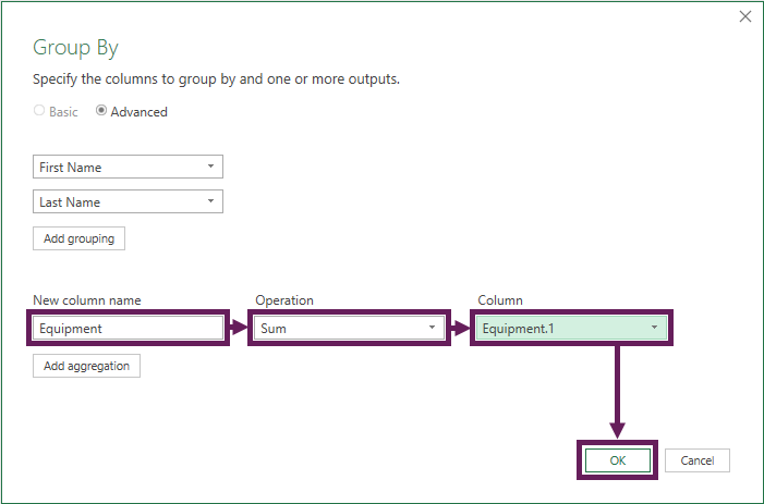
Equipment is a text column, and we have selected the Sum operation. This creates an error, as we cannot sum text.

As you can see above, our column now contains errors.

The operation drop-down has many options: Sum, Average, Median, Min, Max, Count, Count Distinct Rows, and All Rows. Unfortunately, none of these is the option we want.

But don’t worry; we used Sum as a placeholder function, we will fix the error in the next step.

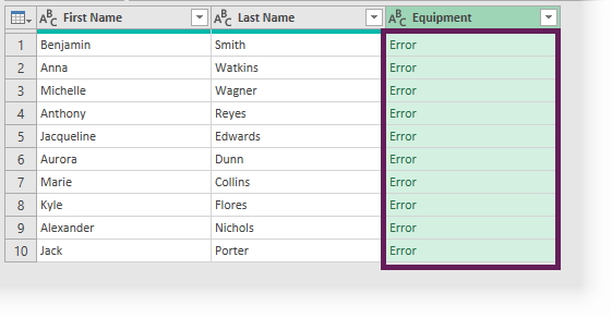
Editing the M Code

Next, we edit the M code in the formula bar to change the List.Sum function for the Text.Combine function.

Hopefully, the formula bar is visible; if not, click View > Formula Bar to enable it.

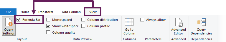
Power Query’s formula bar is similar to the one in Excel. However, the formulas must be M Code rather than standard Excel formulas.

We are using the Text.Combine function to merge the text: https://docs.microsoft.com/en-gb/powerquery-m/text-combine

Text.Combine has the following syntax:

Text.Combine(texts as list, optional separator as nullable text) as text

• Texts: needs to be a list of text strings, which is what we have, because each individual has a list of equipment
• Separator: needs to be the text string used to separate each item

So, if we wanted to separate by a semi-colon ( ; ) and a space character, the formula would be:

Text.Combine([Equipment.1], "; ")

This means in the formula bar, we change the M code from this:

= Table.Group(#"Merged Columns", {"First Name", "Last Name"}, 
    {{"Equipment", each List.Sum([Equipment.1]), type text}})

To this:

= Table.Group(#"Merged Columns", {"First Name", "Last Name"}, 
    {{"Equipment", each Text.Combine([Equipment.1], "; "), type text}})

Now the preview window has reduced each person’s equipment down to a single cell. AMAZING!

Load data into Excel

That’s it. We’re done. Let’s push the data back into Excel.

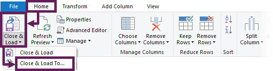
Click Home > Close & Load (drop-down) > Close and Load To…

The Power Query Editor closes, and the view returns to Excel. In the Import Data dialog box, select to load a Table into cell F1 of the existing worksheet.

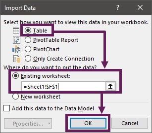
Click OK to close the Import Data dialog box.

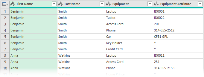
The final data in Excel looks like this:

Power Query merge specific rows

The second scenario occurs when we want to combine specific rows. This typically occurs when there are multiple header rows in our source data. Since Power Query can only have a single header row, we must combine the row text into a single row.

Scenario

Here is the data from the example file.

In the screenshot above, we have multiple header rows. For example, we can see that First and Name are used to describe the cells in column A.

The goal is to concatenate the text into a single row (as shown below).

OK, let’s give this a try.

Convert the data into a Table

Our data is not currently in a Table format. Select any cell in the data and click Insert > Table (or press Ctrl + T).

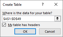
In the Create Table dialog box, ensure the entire data range is included, then click OK.

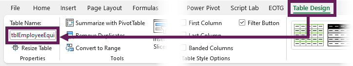
Next, select a cell in the Table. Then, click Table Design > Table Name and provide the Table with a meaningful name. For this example, I have chosen tblEmployeeEquipment.

NOTE: If you do not want to convert the source information into a Table, the alternatives are: (1) create a named range that includes the data, (2) connect to the data from another workbook.

Load the data into Power Query

Select a cell within the Table, then click Data > From Table / Range. The Power Query window opens and shows a preview of the data.

Now we’re ready to start the transformations.

Data preparation

Depending on your default settings, the Applied Steps box may include a step called Changed Type; if so, delete this step. We do not need it.

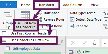
Because our data has come from a Table, the header row is automatically used as the header row in Power Query. We don’t want this, so click Transform > Use first row as headers (drop-down) > Use headers as first row

Transpose, merge columns, transpose

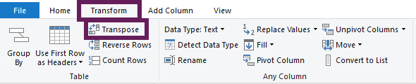
There is no merge rows transformation in Power Query. However, if we transpose data, rows become columns. Which means we can use the merge columns transformation instead.

Click Transform > Transpose.

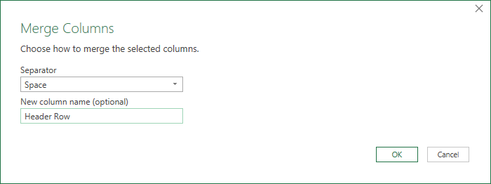
Select Column1 and Column2, then click Transform > Merge columns.

In the Merge Columns dialog box, enter the following:

• Separator: Space
• New Column Name: Header Row

The preview window should display the following:

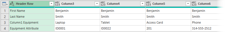
The Equipment column only had a single header row; therefore, the text has been combined with the words Column1 to give a value of Column1 Equipment. Let’s clean that up.

With the Header Row column selected, click Transform > Replace Values. Replace “Column1 ” with blank.

NOTE: Make sure Column1 has a space character after it.

Transpose the data back by clicking Transform > Transpose.

Next, promote headers by clicking Transform > Use first row as headers.

The preview window should look like this. PERFECT!

Load data into Excel

We are done. We can now load the data into Excel. Click Home > Close & Load (drop-down) > Close and Load To…

Using the Import Data dialog box, load a Table into cell F1 of the existing worksheet.

The final data in Excel looks like this:

Conclusion

What would have been complex scenarios for Excel have been made simple with Power Query. However, to combine rows in Power Query takes a slightly different mindset. Therefore, we need to understand the transformations available and how we can join them to achieve the desired results.

Related posts:

• How to split cells in Excel
• Power Query – Split delimited cells into rows
• Power Query – Lookup Values Using Merge

---

What next?

Discover how you can automate your work with our Excel courses and tools.