How to split cells in Excel: 4 simple ways

There are many circumstances where we receive information with multiple data points inside a single cell. This often occurs when the data’s original intention is slightly different from how we intend to use it. In these circumstances, we often need to split a cell into its constituent parts. This post will look at solving this problem and learn how to split cells in Excel.

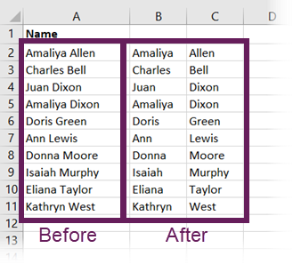
The scenario we are trying to solve is; we want to split an individual’s full name into the first name and last name components.

If we have ten cells, it’s not a big problem; we can do that manually by entering each value into a separate column. But if we have hundreds or thousands of cells, we need to find another way. Thankfully we can turn to a variety of Excel features.

Table of Contents

• Example data
• Split cells using Text to Columns Wizard
• Split cells using Flash Fill
• Background execution
• Manual execution
• Split cells using Power Query
• Split cells using Excel formulas
• Useful Excel functions to split cells
• Example scenario
• Conclusion

Watch the video

Watch the video on YouTube.

Example data

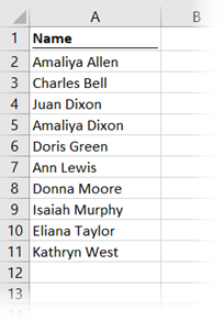
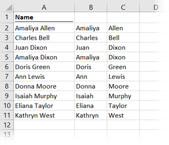
In all our solutions, we will be using the following data set.

In this post, we are covering 4 possible options. Depending on your data, one method may lead to better results than others. The lower the level of data consistency, the harder the process becomes.

Split cells using Text to Columns Wizard

Text to columns is a feature in Excel that hides in plain sight. It’s on the ribbon as an icon, but unless you know it’s there and what it does, you may not have used it before.

The steps to split a cell into multiple columns with Text to Columns are:

1. Select the cell or cells containing the text to be split
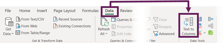
2. From the ribbon, click Data > Data Tools (Group) > Text to Columns
   
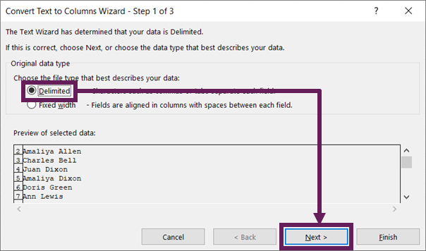
3. The Convert Text to Columns Wizard dialog box will open
4. Select the Delimited option. This allows us to split the text at each occurrence of specific characters. In our case, the space character is our delimiter. Click Next.
   
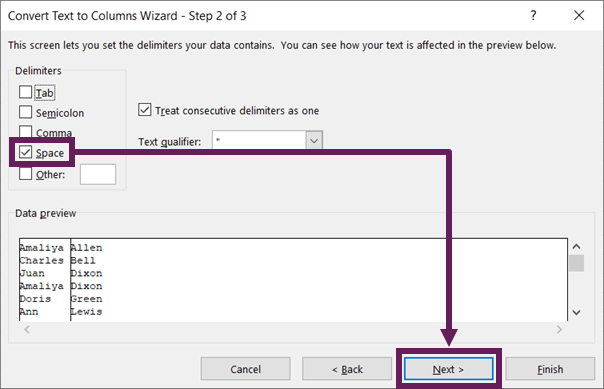
5. Step 2 in the Convert Text to Columns Wizard opens. In the Delimiters group, select the relevant option for your scenario. I have selected Space for this scenario. Click Next.
   
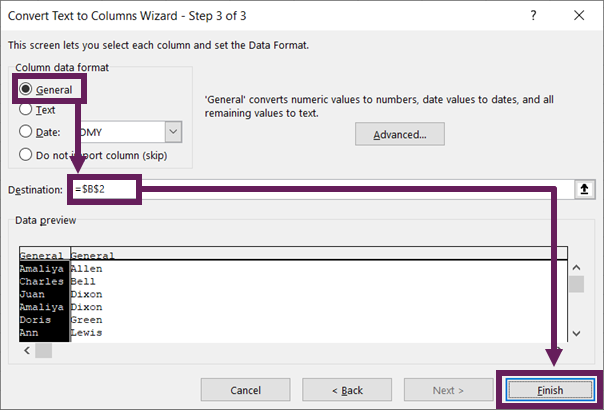
6. Finally, in Step 3 of the Text to Columns Wizard, we specify the format for the result. As we are using text, the General format is a reasonable option. Select a Destination cell where to output the result. I have selected Cell B2. Click Finish.
   

That’s it. Just a few clicks and we’re done 🙂

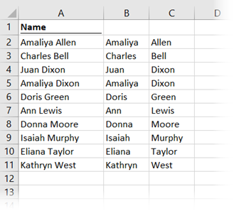
Our range should now be perfectly split into multiple columns.

Split cells using Flash Fill

Flash Fill is a fantastic feature that was introduced in Excel 2013. You may have already used it without even being aware of it. It is very easy to use for splitting cells in Excel with simple patterns.

It can run in two ways:

• In the background, Excel tries to find patterns in the text and automatically makes suggestions.
• Triggered by the user at specific times

Background execution

For background execution:

1. With the source cells on the left, type the text element we want to extract in the first row of the first column (cell B2 in the screenshot below).
   
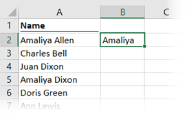
   Nothing will happen yet.
2. Start typing the element of the text we want to extract from the second cell. Now Flash Fill jumps into action and makes recommendations:
   
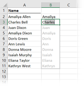
3. Press the Tab or Enter key to accept the recommended fill.

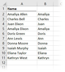
This gives us the first name.

Manual execution

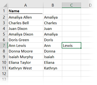
Now let’s manually trigger Flash Fill to get the last name.

1. With the source cells on the left, type the text element to be extracted into any single row.
   
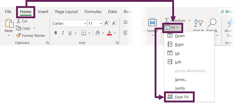
2. Select the cells in the range to be filled with values (cells C2 to C11 in our example), click Home > Fill (dropdown) > Flash Fill.
   

And we’re done. Both first name and last name have been separated into columns. I’ve shown the background and manual methods above; you can use either.

Hopefully, you’ll agree that this future is any quick transformation we may want to make to the cells in Excel.

Split cells using Power Query

Another option for splitting multiple cells in Excel is to use Power Query. This has been natively available since Excel 2016. Prior to that, there was an add-in for Excel 2010 and 2013.

First, let’s load our cells into the Power Query editor.

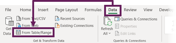
1. Select any cell in the data set, then click Data (tab) > From Table/Range (or Data (tab) > From Sheet in newer versions of Excel) from the ribbon.
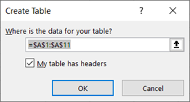
2. If the selected cell is not part of an Excel table already, the Create Table box opens. Ensure the full range is selected, and my table has headers option is checked. Then click OK.
   
3. The Power Query editor will open with all the data displayed.
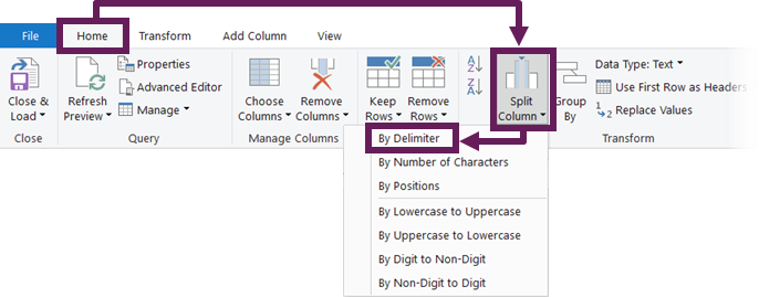
4. From the Power Query ribbon select Home > Split Column (drop-down) > By Delimiter.
   
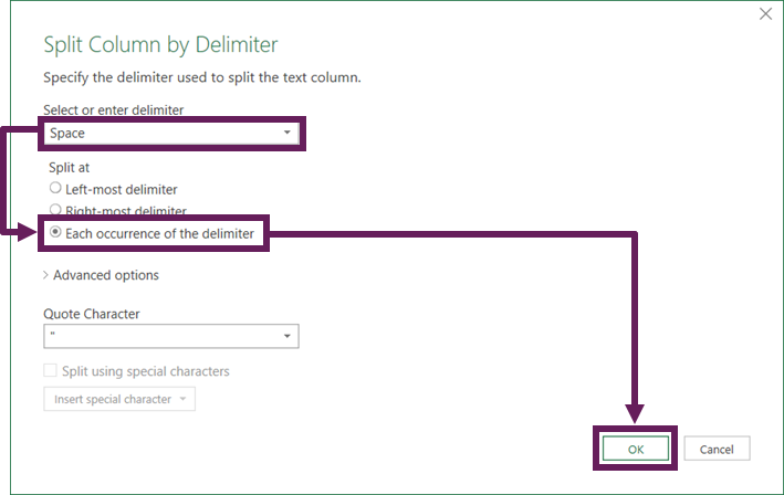
5. Depending on the complexity of your text, there are lots of options to split the contents of a cell by different positions. For our scenario, the Space character and each occurrence of the delimiter are good options. Click OK.
   
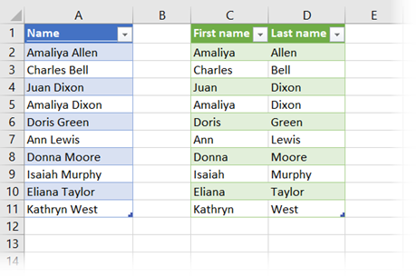
6. In the data preview window, we now have the name split into two different columns.
   
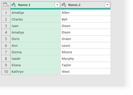
7. In the data preview window, Double click the header and change the headings to First and Last respectively.
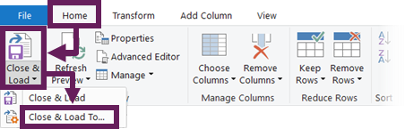
8. Now we need to get the data back into Excel. Click Home > Close & Load (drop-down) > Close & Load To…
   
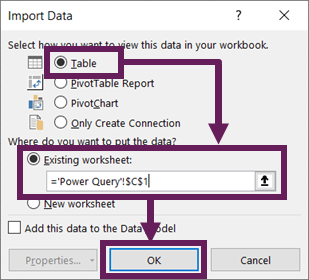
9. From the Import Data dialog box, select Table and choose where to load the information back to. In the example, I have selected an existing sheet at cell C1. Click OK.
   

The transformed data will now be loaded back into the cells in Excel.

Split cells using Excel formulas

In answering the question of how to split a cell in Excel, our final option is to use standard Excel formulas. These give us the ability to split the contents of a cell using any rules we can program into our formulas. While formulas are very powerful, they also require our skill rather than using a point-and-click interface.

Useful Excel functions to split cells

The most useful functions to split multiple cells are:

LEFT

Returns the specified number of characters from the start of a text string.

Example:

=LEFT("Doris Green", 5)

Result: Doris

The second argument of 5 is telling the function to return the first 5 characters of the text “Doris Green”.

RIGHT

Returns the specified number of characters from the end of a text string.

Example:

=RIGHT("Kathryn West", 4)

Result: West

The second argument of 4 is telling the function to return the last 4 characters of the text “Kathryn West”.

MID

MID returns the characters from the middle of a text string, given a starting position and length.

Example:

=MID("Ann Lewis", 5, 3)

Result: Lew

The second argument represents the nth character to start from, and the last argument is the length of the string. From the text “Ann Lewis”, the 3 characters starting at position 5 are “Lew”.

LEN

Returns the number of characters in a text string.

Example:

=LEN("Amaliya Dixon")

Result: 13

There are 13 characters in the string (including spaces).

SEARCH

SEARCH returns the number of characters at which a specific character or text string is first found. SEARCH reads left to right and is not case sensitive.

Example:

=SEARCH(" ","Charles Bell",1)

Result: 8

The space character first appears in the 8th position of the string “Charles Bell”; therefore, the value returned is 8.

The last argument is optional; it provides the position to start searching from. If excluded, the count will start at the first character.

Note: FIND is the case-sensitive equivalent of the SEARCH function.

SUBSTITUTE

SUBSTITUTE replaces all existing instances of a text string with a new text string.

Example:

=SUBSTITUTE("Juan Dixon","Dix","Wils",1)

Result: Juan Wilson

The text string of Dix has been replaced with Wils. The last argument determines which instance to replace. In the formula above, it has replaced the 1st instance only. If we had excluded this argument, it would have replaced every instance.

Example scenario

Our scenario is reasonably simple, to split a cell into multiple columns we can use the LEFT, RIGHT, LEN and SEARCH functions. We can extract the first and last name as follows:

First name:

=LEFT(A2,SEARCH(" ",A2)-1)

• SEARCH finds the space character’s position, which for the first record in the example cells of “Amaliya Allen” is the 8th position.
• We do not want the space character included in the string, so we minus 1 from the result to give us a value of 7.
• LEFT then extracts the first 7 characters of the text string.

Last name:

=RIGHT(A2,LEN(A2)-SEARCH(" ",A2))

• LEN finds the length of the text string, which for “Amaliya Allen” is 13.
• SEARCH finds the position of the space character, which is 8.
• 13 minus 8 provides us with the number of characters after the first space.
• RIGHT is then used to extract the characters after the space.

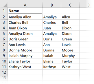
With these two formulas, it gets us back to the same result as we’ve had before; first name in Column B and last name in Column C:

Conclusion

With these 4 techniques, you have learned how to split cells in Excel. Each option has added more and more power to deal with complexity. Which option you choose comes down to your specific scenario. Familiarize yourself with all the options, and then you’ll be able to make the best decisions.

---

What next?

Discover how you can automate your work with our Excel courses and tools.