
In Power Query, when we click the button to combine all the files in a folder, it automatically creates a Transform Sample File for us. Any changes made to the Transform Sample File are applied to all the other files in the folder before they are combined into a single table. This is a really powerful feature; it avoids a lot of very complex M code.
If we connect to a workbook with multiple sheets, wouldn’t it be nice to have similar functionality so we can combine all the sheets in the workbook with a Transform Sample Sheet.
Unfortunately, there isn’t a button on the user interface to achieve this. However, there is a consistent process we can go through to create it ourselves. That is what we are doing in this post.
NOTE: This is one of those processes you need to go through a few times to really understand it. So, make sure to download the example file and work along to see how it all fits together.
Download the example file
Download example file: Join the free Insiders Program to get example files and more.
File name: 0264 Transform sample sheet.zip
Key Information
Framework / Stage: Reporting & Analysis Blueprint / Reshape
Table of Contents:
- Example data
- Connect to the workbook
- How does it work?
- Prepare the query
- Create the Sample Sheet query
- Create the parameter
- Create the Transform Sample Sheet query
- Create the custom function
- Apply the custom function
- Process complete
- Using the TransformSampleSheet
- Conclusion
Example data
For this example, we are importing data from a single workbook called Example Workbook.xlsx. This file contains worksheets called Data 2022, Data 2023, Data 2024 and Data 2025, along with a sheet called Other Sheet.

We do not want to include Other Sheet in our final query.
Each of the 2022 to 2025 worksheet contains values in the following structure

The difference between each sheet is the column headings. Because they each contain dates for different years, it prevents us from easily combining the worksheets.
Connect to the workbook
The first step is to connect to the workbook.
- Open a new Excel workbook.
- From the ribbon, click Data > Get Data > From file > From Excel Workbook.
- Navigate to the location of the Example Workbook.xlsx workbook, select it and click Import.
- In the Navigator window select the Example Workbook.xlsx folder and click Transform Data.
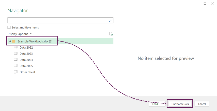
The workbook loads into the Power Query interface with a separate row for each sheet.

How does it work?
Before we go any further, let’s understand how the Transform Sample Sheet process works.
We use the first sheet as a sample sheet that represents all the other sheets in the workbook. Based on the transformations to that sample sheet, we create a custom function.
The transformations and function are tied together. Any new transformations are automatically applied to the function.
Then, we simply apply the custom function to all the sheets in the workbook and combine them together.
Prepare the query
Before we can start creating the additional queries, we need to prepare the existing data with the following steps.
Rename the query
By default, the query will be named based on the workbook name. For our example, let’s rename the query to Combined Data.
Retain only the sheets to combine
Workbooks contain sheets of different types. We only want to combine the sheets which contain the data. In our example, those sheet names all start with the word Data. Let’s retain only those sheets.
- Click the filter button at the top of the Name column, select Text Filters > Begins With….
- In the Filter Rows dialog box, set Begins with to Data.
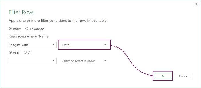
- Click OK.
Everything is ready, we can start building our queries.
Create the Sample Sheet query
The first stage is creating the Sample Sheet query.
- In the Queries pane, right-click on the Combined Data query and click Duplicate. This creates a new query.
- Rename the new query to SampleSheet.
- In the formula bar click the fx icon to create a new step.
- Enter the following code:
= #”Filtered Rows”[Data]{0}
Filtered Rows is the name of the previous step. Change this step name for your scenario.
- Depending on your settings Power Query may create the Promoted Headers and Changed Type steps automatically. If it has, delete both of these steps.
Create the parameter
The second stage is creating the parameter.
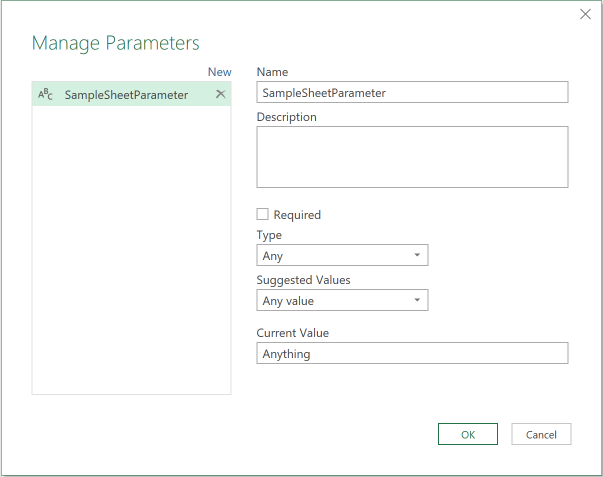
- From the ribbon, click Home > Manage Parameters (Drop Down) > New Parameter
- In the Manage Parameters dialog box:
- Name the parameter SampleSheetParameter.
- Uncheck Required.
- Ensure the Type is Any.
- For the Current Value, enter Anything; this is a placeholder, we will change it next.
- Click OK.
- Let’s edit the code in the parameter. Click Home > Advanced Editor.
- In the Advanced Editor dialog box:
- Replace the placeholder text of “Anything” with SampleSheet.
- Click OK.

Create the Transform Sample Sheet query
The third stage is creating the Transform Sample Sheet query.
- In the Queries pane, right-click on the SampleSheetParameter, select Reference.
- This creates a new query. Rename the query to TransformSampleSheet.
The TransformSampleSheet query displays the data from the first sheet in the workbook.
Create the custom Function
The fourth stage is creating the custom function.
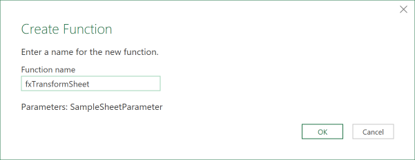
- Right-click on the TransformSampleSheet query and click Create Function… from the menu.
- In the Create Function dialog box, give the function the name of fxTransformSheet.
- Click OK.
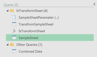
Power Query automatically creates a group which contains the SampleSheetParameter, fxTransformSheet and TransformSampleSheet. Drag the Sample Sheet into the group too.
Any changes made to the TransformSampleSheet are automatically reflected in the fxTransformSheet function.
Apply the custom Function
We are now ready to use the custom function in the Combined Data query.
- Select the Combined Data query.
- Click Add Column > Invoke Custom Function.
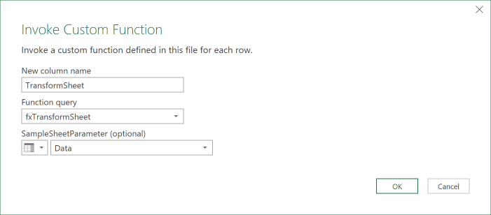
- In the Invoke Custom Function dialog box:
- Set the new column name as TransformSheet.
- Select fxTransformSheet from the function query list.
- Select Data from the SampleSheetParameter list.
- Click OK.
- Select the Name column, hold Ctrl and select the TransformSheet column.
- From the ribbon, click Home > Remove Columns (drop down) > Remove Other Columns.
- Expand the TransformSheet column by clicking the double headed arrow in the column header.
- Uncheck the Use column names as prefix option, click OK.
Power Query combines all the sheets in the workbook into a single table. However, we are not finished yet. If we look at the formula bar, we notice it hardcoded the column names. We need to fix this by editing the M code.
Change the M code to be the following:
= Table.ExpandTableColumn(#”Removed Other Columns”, “TransformSheet”, Table.ColumnNames(TransformSampleSheet))

Instead of hardcoding column names, this code references the column names from the TransformSampleSheet query.
Process complete
That completes the process; we have set up a Transform Sample Sheet. Any changes we make to the TransformSampleSheet query are incorporated into the fxTransformSheet function, which is then applied to all the sheets in the workbook.
Let’s test it out in the next section.
Using the TransformSampleSheet
Let’s make some changes to the TransformSampleSheet and ensure they flow through into the Combined Data query.
The key to success with this method is any column names hardcoded into the TransformSampleSheet query must exist in all the sheets. Therefore, as we make transformations, we need to pay close attention to the formula bar to ensure we achieve this.
This example assumes we have default settings applied. If you don’t have the default settings, then you may not need all the steps.
- Select the TransformSampleSheet query.
- Click Home > Remove Rows > Remove Top Rows.
- In the Remove Top Rows dialog box:
- Set the number of rows to 3.
- Click OK.
- Select the Column1 column and click Home > Remove Columns.
- Click Home > Use First Row As Headers to promote the headers.
- Delete the auto-applied Changed Type step.
- Right-click on the word Total in the last row of the Item column, select Text Filters > Does Not Equal from the menu.
- Select the Item column, hold shift, select the Size column.
- Click Transform > Unpivot Columns (drop down) > Unpivot Other Columns.
- Rename the Attribute column to Date.
- Apply Data Types as follows:
- Item: Text.
- Size: Text.
- Date: Using Locale…
- Data Type: Date.
- Locale: English (United Kingdom) .
- Click OK.
- Value: Decimal Number.
The data in the Transform Sample Sheet is now in a good data layout.
If we look in the Advanced Editor, we see our transformations only reference columns that exist in all of the sheets or created by the process. Therefore, this transformation will not cause any errors.
If we go back to the Combined Data query, we see these transformations are applied to all our sheets, and we now have a perfect dataset to load into Excel.
Conclusion
In this post, we have seen how to create a Transform Sample Sheet in Power Query. It takes a few steps to setup the first time, but the good news is that those steps can be replicated over and over. The best news of all is that this can save us from a lot of complex M code.