
One of the first things we learn in Excel is the magic of the $ symbol. It freezes the row or column, so the cell reference does not change when copying a formula. This is known as an absolute reference. With the introduction of Tables came a different (and more semantic) way to reference cells, called structured references. However, structured references don’t follow the same principles as the standard A1 style referencing system we usually use. As a result, the $ symbol approach won’t work. But don’t worry; by the end of this post, you will know how to create an Excel Table absolute reference.
Table of Contents
Download the example file: Join the free Insiders Program and gain access to the example file used for this post.
File name: 0122 Excel Table absolute reference.xlsx
Watch the video

Scenario
The examples in this post all use the following Table.
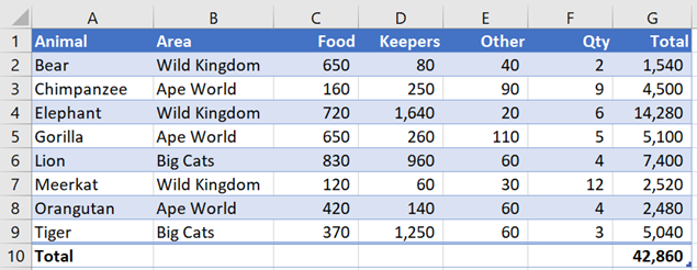
The Table shows the costs a Safari Park might incur for owning different types of animals. The Table name is myTable, whilst it’s not a great name, it will work for this example.
Excel Table absolute reference for column
When using structured references, whole columns are referenced with this syntax:
tableName[columnName]Using the example data to sum the Total column, the formula would be:
=SUM(myTable[Total])If this were dragged or copied to another column, the formula would change automatically. If copied to the left, it would change to:
=SUM(myTable[Qty])If copied to the right, it would revert to the first column in the table and changes to:
=SUM(myTable[Animal])NOTE: This is one of the quirks when working with Table columns. Once a structured column reference reaches the end of the Table, it loops back to the start.
If using the standard A1 style referencing, we could add the $ signs and change the range from G2:G9 (a relative reference) to $G$2:$G$9 (an absolute reference). But we can’t use $ with the structured references found in Tables.
To achieve the same result, we need to add more square brackets, a colon ( : ), and repeat the column name.
=SUM(myTable[[Total]:[Total]])The difference between the relative and absolute reference for columns is shown in blue above.
If you have been using Tables for a while, you will notice this is the same syntax as when referencing multiple columns.
=SUM(myTable[[Food]:[Other]])The reference above shows how to sum the columns from Food to Other in the example data. This means multi-column references selected using the mouse are absolute by default.
To create a relative multi-column reference, we need to remove the outer square brackets and repeat the table name, as shown below.
=SUM(myTable[Food]:myTable[Other])Or you could include each column individually within the calculation as shown below, which achieves the same result.
=SUM(myTable[Food],myTable[Keepers],myTable[Other])Relative and absolute reference for cells in the same row
When using Tables, the syntax to reference a cell in the same row is as follows.
=[@Total] or =[@[Total Value]]NOTE: the 2nd syntax in the example above is where the header contains a space or special character.
If the formula is contained in a cell outside the Table, the Table name must also be added:
=myTable[@Total] or =myTable[@[Total Value]To make a row reference absolute, the same principles apply as we saw for column references. It does not matter if the reference is inside or outside the Table; the Table name is required for both.
=myTable[@[Total]:[Total]]To reference multiple columns, the syntax is similar.
=SUM(myTable[@[Food]:[Other]])The reference above shows how to sum the columns from Food to Other from the example data. This is an absolute column reference.
To create a relative multi-column reference, we need to remove the outer square brackets.
=SUM([@Food]:[@Other]) or =SUM(myTable[@Food]:myTable[@Other])NOTE: The @ symbol serves the same purpose as when working with dynamic arrays; it calculates based on the implicit intersection. Check out this post for more information: Dynamic arrays in Excel
Relative and absolute reference for any cell
In the section above, we considered the scenario where the column was absolute while the row was based on a cell in the same row. However, to reference a row which is not in the same row different approach.
The INDEX function returns a cell reference or value from a specified location in a range or array. As a simple example, look at the following formula:
=INDEX($G$2:$G$9,1)This formula would always return the first row from cells G2:G9. To return the second cell from the same range, the formula would be
=INDEX($G$2:$G$9,2)
Therefore, using INDEX with structured references allows us to refer to any individual cell in the range. For example, the following returns the first item from the Total column.
=INDEX(myTable[Total],1)Tow is an absolute reference, but the column is relative; therefore this is a mixed reference.
To create a full relative reference, we must also find a way to count row numbers within the INDEX.
The following uses ROW(A1) to calculate a relative row reference. ROW(A1) evaluates to 1. When dragged down, ROW(A2) evaluates to 2. Therefore ROW creates the relative number to use in the INDEX function.
=INDEX(myTable[Total],ROW(A1))The formula above is a fully relative table reference.
Absolute references in Headers and Totals
Referencing the Header and Total rows within a Table is slightly different again. This is because Headers and Totals inherently have absolute row references but not column references.
The relative reference for Headers is shown below:
=myTable[[#Headers],[Food]]To turn the Header reference into an absolute reference, add the section highlighted below.
=myTable[[#Headers],[Food]:[Food]]If you’ve read this post all the way through, then the multi-column absolute reference will not surprise you. The formula to count the column headings is shown below.
=COUNTA(myTable[[#Headers],[Food]:[Other]])And the multi-column relative reference will not surprise you either.
=COUNTA(myTable[[#Headers],[Food]]:myTable[[#Headers],[Other]])The examples in this section all include the Header row (#Headers). To reference the Total row, use #Totals instead.
Conclusion
With a Table, the different syntax to provide relative or absolute references can be quite subtle. An @ or square bracket out of place can cause an error that can be incredibly frustrating to find. It is easier to start with a valid reference and then adjust it, rather than typing the reference from scratch.
As with all things, practice is vital. Before long, creating an Excel Table absolute reference will be second nature.
Related posts:
Discover how you can automate your work with our Excel courses and tools.
The Excel Academy

Make working late a thing of the past.
The Excel Academy is Excel training for professionals who want to save time.
Is it possible to reference by numbers rather than by name? Thx! KR!
Hi Sunny – I don’t believe there is a way to do that with structured references. That’s not what the tables feature in Excel was intended for.
Yes @sunny.
If you wanted to get the column # to use in a formula like VLOOKUP which requires an INDEX #, you could do something like this:
COLUMNS(myTable[[#Headers],[Animal]:[Keepers]],FALSE)
Would return 4. What is valuable in this way of referencing the index # is that if you add columns to a table, you don’t have to update absolute index numbers. Also, if you rename the column in your table, all formulas referencing that table column name are updated as well.
Cheers,
-.Mark
Hi,
I have a table (Table1) with 5 columns.
What I want is to get the value of a single cell on one of the 5 columns.
Following is working, but i was asking myself if there is an other way to do it.
=INDEX(Table1[Arsenal];10)
i was thinking on something like:
=Table1[Column Name],[Row Number]
Best regards
Hi Ludo – to my knowledge, there is no method for referencing a cell in a table using structured references. You would need a formula, such as INDEX to achieve that.
Is there a way to lock the column reference with a keyboard shortcut like F4? I had to update some formulas by typing it and I would prefer a faster way.
I wish there were, it would be amazing. Unfortunately, we are left to enter the [] by ourselves.
One option is to select multiple columns to get the correct syntax, then change the column name. I find this easier than selecting one column and then creating the correct syntax. 🙂
Of course, within the table, you could always ignore Excel’s helpfulness & still use the $Column$Row format for any fixed references
But that breaks the entire construct of using Structured Reference. Therefore the auto expansion and calculated columns features of the Table aren’t guaranteed to work properly.
Using ROW(A1) in an index formula the way you did is dangerous, because inserting a row above row 1 will change it to ROW(A2) and break it.
However, using ROW(A1)+1-ROW($A$1) works, since inserting a row changes it to Row(A2)+1-ROW($A$2).
That is a very valid point.
In reality I can’t think of many scenarios where this would be required. We generally need the first, which is INDEX(tableName[columnName],1), or the last which INDEX(tableName[columnName,ROWS(tableName))
Copying to the right behaviour depends on how you perform the action.
Using the drag handle implies a relative reference to a column, while Ctrl+R implies an absolute reference to a column. Maybe this will help some people?