How to use Excel Table within a data validation list (4 easy ways)

Excel Tables expand automatically whenever new data is added. This feature alone makes Tables one of the most powerful tools within the Excel user’s toolkit. A Table can be used as the source data for a chart and within a named range, both of which benefit from the auto-expand feature. Data validation lists would also benefit from the auto-expand feature, but they just don’t work correctly—an oversight on Microsoft’s part (in my opinion).

In this post, we examine the issues and solutions for creating an Excel data validation list from a Table.

Table of Contents

• Example data
• The problem
• Normal cell references over a Table
• Problems with this approach
• INDIRECT function
• Warning about this method
• Named range of the Table column
• Create the named range
• Add the named range to the data validation list
• Key points about this method
• Dynamic array spill range
• Create a spill range
• Use the spill range in the data validation list
• Key points about this method
• Which method to choose?
• Conclusion

Example data

The examples in this post use the following data:

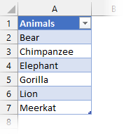
The Table name is myList (I know, it’s not a great name, but it will work for the examples).

The problem

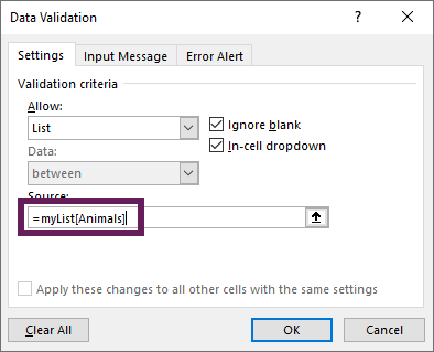
The following data validation settings look like they should work. It should use the column called Animals from a Table called myList.

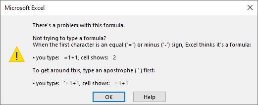
Instead of giving us an Excel data validation list from the Table, Excel shows an error message.

What can you use to solve this problem? I’ve got four solutions for you:

• Normal cell references over a Table
• INDIRECT function
• Named range of the Table column
• Dynamic array spill range

Let’s look at each of these and you can decide which is the best option for your situation.

Normal cell references over a Table

Normally, if we use standard cell references, the data validation list is static. Each time a new item is added to the list either the data validation source will need to be updated, or the new items will need to be added within the existing list range.

However, if we create the data validation list using normal cell references, which also happen to be all the rows from a Table column, it will expand.

Look at the screenshot below. The cells $A$2:$A$7 are exactly the same cells as the reference myList[Animals] would be for a Table.

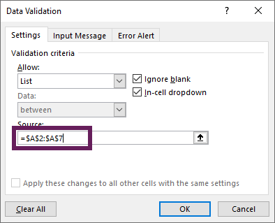
It looks like it would behave like a standard static list. But somehow Excel knows.

If we add data to the bottom of the Table, the data validation list expands when values are added to the Table. Try it for yourself.

Problems with this approach

Now, don’t get too excited. There is a big problem with this approach:

1. If the data validation list is on a separate sheet to the Table, it does not expand.
2. This method only works if the cells selected include the entire Table column (i.e., in our example, if you reference $A$4:$A$7 it will not expand when a new item is added as it is not the whole Table column).

Due to the issues noted above, it is probably best to avoid this method.

INDIRECT function

The INDIRECT function converts text into a Range that Excel recognizes and can use in calculations. For example, if Cell A2 contains the text “A1” you can write =INDIRECT(A2) and Excel converts that to the cell reference =A1.

We can use the INDIRECT function with the Table and column reference as text and Excel will understand this.

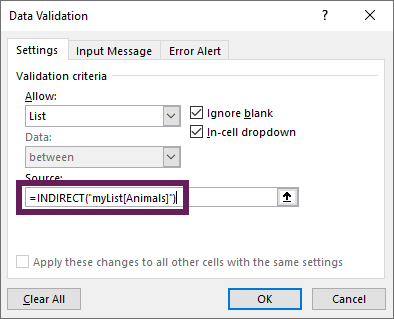
The formula used in the screenshot above is.

=INDIRECT("myList[Animals]")

If the list only has one column, it is possible to refer to just the Table.

=INDIRECT("myList")

The range for the data validation list now expands whenever new items are added to the Table.

Warning about this method

With this method, there is one key thing to be aware of; the Table and column names are hardcoded into the INDIRECT formula. If either of these change, the data validation list will cease to work as the formula cannot find the source data.

Named range of the Table column

Named ranges accept a Table column as the source, and data validation lists accept a named range. Therefore, we can take a two-step approach to achieve the desired result.

Create the named range

To create the named range, click Formulas > Define Name

The New Name dialog box opens.

Give the named range a name (myDVList in the example below) and set the Refers to box to the name of the Table and column.

Click OK. The named range has been created.

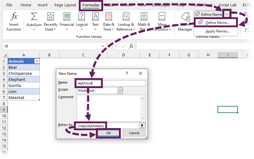
The formula used in the screenshot above is.

=myList[Animals]

As with the example above, if the Table only has one column, we can refer to just the Table without the column name.

Add the named range to the data validation list

The screenshot below shows the named range added to the data validation list box.

The data validation list now expands whenever new items are added to the Table.

Key points about this method

In relation to this method, there are a few things to be aware of:

• This is a two-stage process, which takes a little longer to set up.
• If the Table or Column names change the named range automatically updates to reflect the changes.

While it takes longer to set up, this method is harder to break.

Dynamic array spill range

We are about to get technical for a moment, but don’t worry applying this method is very easy, so stick with me.

Excel 2021 and Excel 365 have a feature known as dynamic arrays. These allow a formula to return multiple results and to spill the results across multiple cells; this is known as a spill range.

If the number of rows returned by the formula changes, the rows and columns in the spill range also change.

We use the # sign (also known as the spill operator) to refer to the cells in the spill range.

Here is the key part… data validation lists accept the spill range as a valid range reference. So this means we can create a two-step process:

• Create a spill range
• Use the spill range in a data validation list

Create a spill range

To create the spill range on a sheet, we just need to refer to the Table and column.

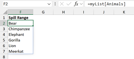
The formula in cell F2 is:

=myList[Animals]

Since the Table column has multiple cells, those values spill down into cells F2:F7. This can be seen by the blue box which highlights the spill range.

If the number of items in the Table changes, the spill range of the Table changes.

Just as for previous methods, if the Table only contains a single column, we could refer to just the Table name of myList, instead of the myList[Animals].

Use the spill range in the data validation list

To get the spill range into the data validation list, we refer to the first cell in the range, followed by #.

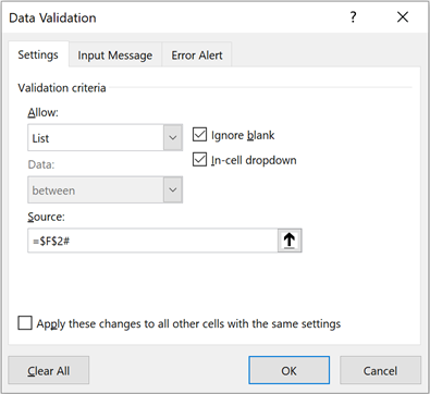
In the screenshot above, we are using cell F2 and its spill range as the source for the data validation list.

If the data validation list refers to the range on another worksheet, the sheet name must also be included in the source, such as:

='Sheet Name'!$F$2#

Key points about this method

In relation to this method, there are a few things to be aware of:

• This is a two-stage process, which takes a little longer to set up.
• If the Table or Column names change, the formulas update automatically to reflect the changes.

Which method to choose?

So, with four options to choose from, the question is which is the best?

I don’t advise using the standard cell references over a table as it won’t work across worksheets. And I avoid the INDIRECT method as it can easily break if renaming Tables or columns.

I like the named range and spill range options. While they take a few extra seconds, they are easy to set up and less likely to break if changes occur.

Conclusion

We cannot create an Excel data validation list directly from a Table. However, in this post, we have seen four methods that we can use to achieve the same result.

Related Posts:

• Don’t trust data validation in Excel!
• How to loop through each item in Data Validation list with VBA
• How to use Table slicers for advanced interactivity in Excel

---

What next?

Discover how you can automate your work with our Excel courses and tools.