VLOOKUP: How to calculate faster

I hardly ever use an approximate match with VLOOKUP due to the risk of getting an incorrect result. But I learned this little trick – which provided almost unbelievable speed increases.

The problem

With a VLOOKUP an exact match (i.e. including FALSE as the last argument) is a slow method of calculation. It will search through each record one-by-one until it finds a match. Using an approximate match (i.e. including TRUE as the last argument) is very fast in comparison, as it does a binary search. An approximate match only works with sorted data but can find the lookup value faster. However, if the lookup value is not in the list it will return an incorrect result.

The solution

This trick involves combining two approximate matches together to return the equivalent of an exact match. If there is no matched value it will return an #N/A result.

An exact match VLOOKUP would be defined like this:

=VLOOKUP(lookup_value, table_array, col_index_num, FALSE)

But combining two VLOOKUP’s to create an equivalent to an exact match looks like this:

=IF(VLOOKUP(lookup_value, table_array, 1, TRUE)=lookup_value,
VLOOKUP(lookup_value, table_array, col_index_num, TRUE),NA())

How does this work?

Let’s break this formula down into understandable sections. First, Let’s consider the first VLOOKUP statement.

=IF(VLOOKUP(lookup_value, table_array, 1, TRUE)=lookup_value,
VLOOKUP(lookup_value, table_array, col_index_num, TRUE),NA())

The section highlighted above carries out an approximate match VLOOKUP calculation on the first column. If it finds an exact match it will return the lookup value, otherwise it will return a different value.

Now, let’s consider the IF statement.

=IF(VLOOKUP(lookup_value, table_array, 1, TRUE)=lookup_value,
VLOOKUP(lookup_value, table_array, col_index_num, TRUE),NA())

The returned value is compared to the original lookup value. If it is the same (i.e. an exact match exists) it will become TRUE, if it is different it will become FALSE.

Finally, let’s look at the second VLOOKUP.

=IF(VLOOKUP(lookup_value, table_array, 1, TRUE)=lookup_value,
VLOOKUP(lookup_value, table_array, col_index_num, TRUE),NA())

Where the value of the first VLOOKUP is TRUE the second VLOOKUP is then calculated. We already know that an exact match exists, so it will return the correct value from the column number identified.

The benefit

This formula may seem like an over-complication. If your worksheet is calculating quickly, then Yes, it probably is. However, a slow calculating worksheet can waste a lot of time. So, if your worksheet is slow, this formula can create significant speed benefits. Even though the new formula is carrying out two VLOOKUPs and an IF, the calculation speed is still much faster than a single exact match VLOOKUP.

I carried out a few speed tests. Using 100,000 lines of unique data, I timed a VLOOKUP to find 5,000 lines matching lines. Average times over 5 tests were:

	Seconds
Exact Match	14.6107
Combined Approximate Match	0.0267

Wow! That’s over 500 times faster! 500 times faster!! That is equivalent to an 8-minute calculation being reduced down to just 1 second. Don’t tell me you’re not blown away by this, because I was.

Jeff Weir at Daily Dose of Excel has carried out even more tests to find fast this trick is. Check out his post, as it is very interesting, especially the chart comparing speed as the volume of data increases.

Conclusion

Are you are using a lot of VLOOKUPs? Is the calculation speed feeling a bit sluggish? If so, sort your data and switch to this VLOOKUP combination with approximate matches. You will see an instant speed boost. I can’t guarantee it will be the same speed boost I obtained, but you should definitely see a speed increase.

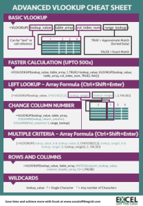
Download the Advanced VLOOKUP Cheat Sheet

Download the Advanced VLOOKUP Cheat Sheet. It includes most of the tips and tricks we’ve covered in this series, including faster calculations, multiple criteria, left lookup and much more.

Please download it and pin it up at work, you can even forward it onto your friends and co-workers.