AGGREGATE: The best Excel function you’re not using

In Excel 2010, Microsoft introduced a new function called AGGREGATE. It is one of the most powerful functions in Excel, yet I’ve rarely seen it used in a real-life scenario.  My aim with this post is to show you how good AGGREGATE is, so that you can make use of its power.

What does AGGREGATE do?

Its name is deceptive. What does the word aggregate mean? To form a whole from separate parts.  That sounds the same as SUM doesn’t it?  Hence the problem with its name, the AGGREGATE function does so much more than SUM.

AGGREGATE can COUNT, AVERAGE, MAX, SMALL and SUM, to name just a few.  But it’s better than those functions because it performs all of those whilst ignoring errors, hidden cells and other cells containing AGGREGATE  and SUBTOTAL functions.

To help you see the power, let’s consider some scenarios.

Scenario 1

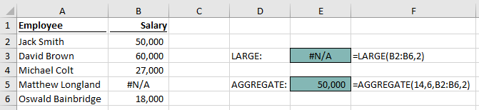
Let’s say you want to find the 2nd largest result over a range of cells where those cells contain an #N/A error.  We would typically turn to the LARGE function for this type of calculation, but in this circumstance, LARGE will return an error.

We can tell the AGGREGATE function to ignore the error,  enabling it to calculate the correct result.

The screenshot below shows the result of both the LARGE and AGGREGATE functions.

Scenario 2

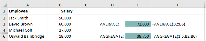
As a second example, what if you want to find the average of the visible cells.  The AVERAGE function will calculate using all the cells in the range; it does not care whether those cells are visible or not.

We can tell the AGGREGATE function to ignore hidden cells, enabling it to calculate the correct result.

The screenshot below, in which row 5 is hidden, shows the average of the visible cells should be 38,750 (as calculated by AGGREGATE), not 71,000 (as calculated by AVERAGE).

Bonus feature

As a bonus, AGGREGATE can also process arrays for specific functions without the need for Ctrl + Shift + Enter. If you don’t know what that means, don’t worry. But if you do, you’ll know this is a big deal.

How to use AGGREGATE

The AGGREGATE function can have two syntax forms:

Reference form:

=AGGREGATE(function_num,options,ref1,[ref2],...)

Array form:

=AGGREGATE(function_num,options,array,[k])

You do not need to worry about which form you are using.  Excel will adopt the necessary form based on the function_num selected.

Let’s consider each of the arguments in the function.

function_num

A value from 1 to 19 which indicates the type of action to be performed.

function_num	Calculation performed	Description	Function Form
1	AVERAGE	Returns the average (mean)	Reference
2	COUNT	Counts number of values or cells which contain numbers	Reference
3	COUNTA	Counts number of values or cells which are not empty	Reference
4	MAX	Returns the largest value	Reference
5	MIN	Returns the smallest value	Reference
6	PRODUCT	Multiplies all the numbers	Reference
7	STDEV.S	Estimates standard deviation based on a sample	Reference
8	STDEV.P	Calculates standard deviation based on a population	Reference
9	SUM	Adds all the values or cells in a range	Reference
10	VAR.S	Estimates the variance based on a sample	Reference
11	VAR.P	Calculates variance based on a population	Reference
12	MEDIAN	Returns the median (the number in the middle)	Reference
13	MODE.SNGL	Returns the most frequently occurring number	Reference
14	LARGE	Returns the nth largest value	Array
15	SMALL	Returns the nth smallest value	Array
16	PERCENTILE.INC	Returns the nth percentile of values in a range which includes the value	Array
17	QUARTILE.INC	Returns the quartile based on a percentile including the value	Array
18	PERCENTILE.EXC	Returns the nth percentile of values in a range which excludes the value	Array
19	QUARTILE.EXC	Returns the quartile based on a percentile excluding the value	Array

options

A value from 0 to 7 indicating the cells to include within the function

options	Description
0 or [blank]	Ignore nested SUBTOTAL and AGGREGATE functions
1	Ignore hidden rows, nested SUBTOTAL and AGGREGATE functions
2	Ignore error values, nested SUBTOTAL and AGGREGATE functions
3	Ignore hidden rows, error values, nested SUBTOTAL and AGGREGATE functions
4	Ignore nothing
5	Ignore hidden rows
6	Ignore error values
7	Ignore hidden rows and error values

ref1 /  [ref2]

ref1: a reference to the range of cells on which the function is to be applied

[ref2]: an optional additional range of cells. There can be up to 252 separate ranges (including ref1), each separated by a comma ( , ).

array

An array of values or an array formula upon which the function is to be applied

[k]

A selection criteria which applies to specific function_nums

calculation	Description
LARGE	The nth largest value to be found
SMALL	The nth smallest value to be found
PERCENTILE.INC	The percentage value, must be between 0 and 1
QUARTILE.INC	The quartile, must be 0, 1, 2, 3, 4
PERCENTILE.EXC	The percentage value, must be between 0 and 1
QUARTILE.EXC	The percentage, must be 0, 1, 2, 3, 4

Too many things to remember?

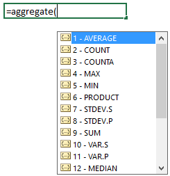
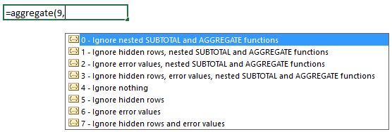
If you think that AGGREGATE is complicated because there are too many things to remember, don’t worry.   When you start typing the function into a cell or in the formula box, a drop-down will appear with the various options.

The function_num drop-down list

The options drop-down list

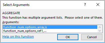
If you decide to apply the function through the fx button, it is much less helpful.

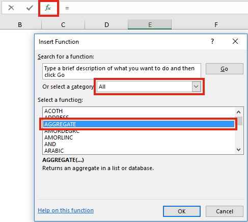
It requires you to select the format of the of the function (though if you select the wrong form and apply the arguments in the right positions, it will still calculate correctly).

The Function Arguments Window does not provide any guidance on the function_num or options.

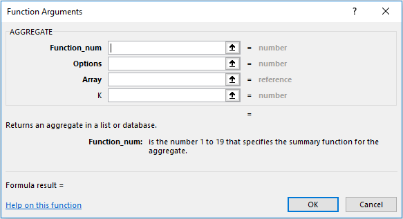
Therefore, to use the AGGREGATE function, it is best to type directly into the cell or formula box, rather than using the fx button.

Examples

Now that you understand the function a bit, we can start to look at a few examples.

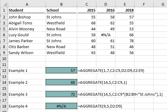
Notice that row 4 is hidden and Cell D6 contains an error.

Example 1 – Multiple references

The formula in Cell B12 is:

=AGGREGATE(1,7,C2:C9,D2:D9,E2:E9)

This formula is calculating the average (function_num = 1) of cells C2-C9, D2-D9 and E2-E9 whilst ignoring hidden rows and errors (options = 7).

Whilst it is possible to include a single reference of C2:E9, this example shows each column of values individually.

Example 2 – LARGE

The formula in Cell B14 is:

=AGGREGATE(14,5,C2:C9,1)

This formula is calculating the 1st largest (function_num = 14) value in the Range C2-C9 whilst ignoring hidden rows (options = 5).

Example 3 – LARGE array formula avoiding Ctrl + Shift + Enter

This example is much more complex.  If you do not understand what it means, don’t worry.  You can still use AGGREGATE without understanding this example.

The formula in Cell B16 is:

=AGGREGATE(14,5,C2:C9*(B2:B9="St Johns"),1)

This example is an extension of Example 2 above.  It now includes the requirement that 1st largest only be calculated over students from the St Johns school.

If we tried to achieve the same result with the standard LARGE function we would need to press Ctrl + Shift + Enter, because it is an array formula.  An example can be seen below, do not enter the curly braces, Excel will add those itself.

{=LARGE(C2:C9*(B2:B9="St Johns"),1)}

AGGREGATE does not need Ctrl + Shift + Enter to be used when using the function_num 14  to 19.

Before you get too excited, there is an issue here.  How is it possible that the largest value for St Johns is 72 when in Example 2 the largest value for all schools was 68?

This is a quirk of array formulas.  The 72 returned for St Johns is contained within the hidden row.  We selected option 5 to ignore hidden rows, but this setting has been ignored.

The problem is the calculation chain.  Excel will evaluate the formula in the following order:

1. B2:B9=”St Johns” = {TRUE;FALSE;TRUE;FALSE;TRUE;TRUE;FALSE;FALSE}
2. C2:C9*{TRUE;FALSE;TRUE;FALSE;TRUE;TRUE;FALSE;FALSE} = {55;0;72;0;58;60;0;0}
3. =AGGREGATE(14,5,{55;0;72;0;58;60;0;0},2)
4. =72

The array part of the function is calculated first, turning the cell references into values.  As a result, there are no cell references to ignore.  This is not necessarily a calculation error; we just need to understand how the formula works.

Example 4 – Without ignoring errors

The formula in Cell B18 is:

=AGGREGATE(9,5,D2:D9)

This formula is trying to SUM (function_num = 9) the values, in Cells D2:D9 whilst ignoring hidden rows (options = 5).   The result of the formula is an #N/A error because the cells included also include an error.

Common errors / problems

As with all functions, there are some common pitfalls and problem.

• If a [k] argument is required, but not provided a #VALUE error will appear. For example, when applying the LARGE function_num, there needs to be an argument to find the nth largest item.
• Whilst there is an option to ignore hidden rows, there is no option to ignore hidden columns.
• When using an array which involves a calculation, the ignore hidden rows option is ignored (as shown in Example 3 above).

If it’s good, why not use AGGREGATE all the time?

If I have convinced you that AGGREGATE is a fantastic formula, then why not use it all the time?

There are a few drawbacks:

• It’s more complicated to use than it’s standard counterpart (i.e., SUM is easy to use, but to summing with AGGREGATE is a bit tricker)
• Takes longer to input all the arguments
• Too many options to remember
• Most users do not understand the function.
• Will not work for users with Excel 2007 or before

But there are just as many good reasons to use it too.

• Can do 152 different things (19 functions x 8 options), rather than just 1 (it’s a Swiss Army knife formula).
• Don’t need to fix formula errors in the range used within the function
• Calculations can be performed on the visible cells of filtered lists
• Can handle array formulas for specific function_num’s
• It’s a very fast formula

There you have it, that’s AGGREGATE, the best function you’re not using . . . until today.

---

What next?

Discover how you can automate your work with our Excel courses and tools.

The Excel Academy