How to list all possible combinations from multiple lists (2 ways)

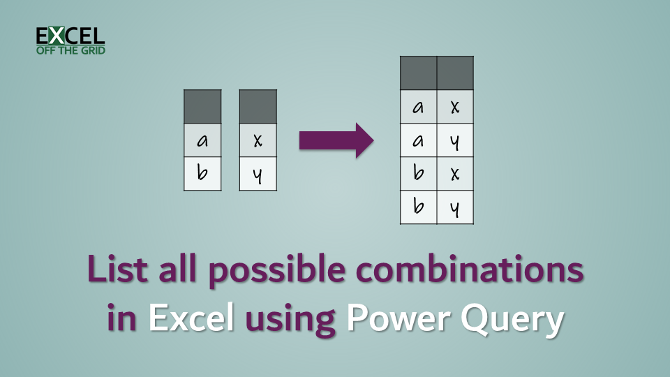
Imagine a scenario where you have two or more lists in Excel and from that, you want to list all possible combinations in one table. This is known as a cartesian join. The question might come in a simple form, such as: “How can we get a complete list of all General Ledger and Cost Centre combinations?”. Sounds simple, right? There must be a single function in Excel or Power Query that will generate that… right?

Er, actually… No. We’ll need to get a little more involved. Let’s dig into Power Query to see how we can solve this problem.

In this post, there are two solutions presented. They each teach us different things about Power Query, so it’s worth working through both and understanding the differences.

Table of Contents

• Load the data into Power Query
• Option #1: Merging tables
• Option #2: Working with tables
• Conclusion: List all possible combinations

Watch the video:

Watch the video on YouTube

Load the data into Power Query

Both solutions in this post require data to be loaded into Power Query. So let’s start there.

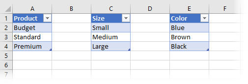
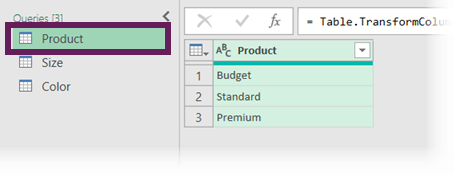
The example file contains 3 tables:

• Product
• Size
• Color

First, we need to load all three tables into Power Query.

1. Select a cell with the table
2. Click Data > From Table/Range
   
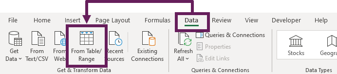
3. The Power Query editor will open with the selected data loaded.
   
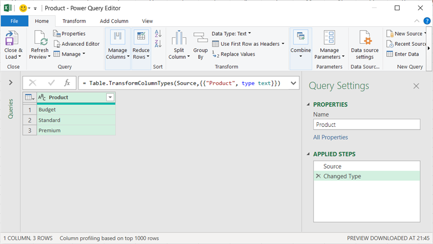
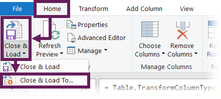
4. Next, we need to load the data as a connection only. Click Home > Close & Load > Close and Load To….
   
   
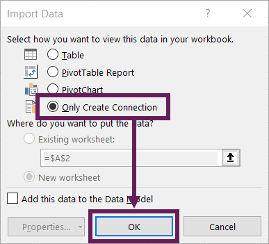
5. The Import Data dialog box will open. Select the Only Create Connection option, then click OK.
   

Repeat these steps for each table.

Option #1: Merging tables

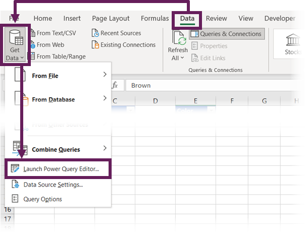
Once all 3 tables have been loaded, go back into the Power Query editor by clicking Data > Get Data (dropdown) > Launch Power Query Editor.

The first option uses Power Query’s merge feature. However, before we can use that, there is another step we must undertake to prepare the data.

1. Select the first query.
   
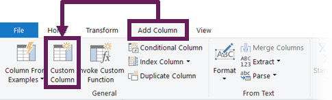
2. Click Add Column > Custom Column from the ribbon.
   
3. In the Custom Column dialog box, enter the following information:
   New Column Name: Temp
   Custom column formula: =1
   The Custom Name and Column Formula can be any value you wish. But in this example, I’ve used these values.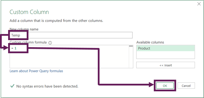 
   
   Then click OK.

Repeat the steps above for each query. Make sure the Custom Column name and Custom Column formula are identical across all the queries.

Our preparation is complete, so we can move on to merging the queries.

1. Click Home > Merge Queries (dropdown) > Merge Queries as New.
   
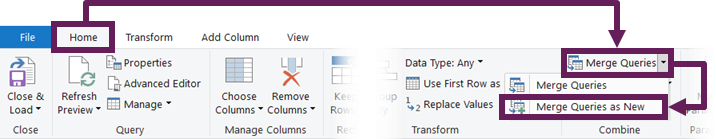
2. The Merge dialog box will open.
   Select two separate lists in each section.
   Click the Temp column (or whatever name you chose) in both lists.
   Set the Join Kind to be Full Outer (all rows from both)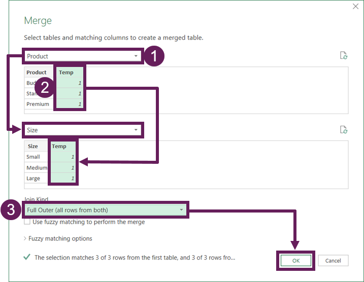
   
   Then click OK.

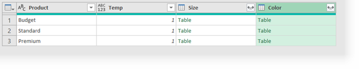
Now merge any additional tables into the existing merged table.

Your Power Query window will look similar to this.

To create the list of all possible combinations:

1. Click the Expand button in the column header.
   From the sub-menu:
   Select only the column with the data we wish to retain (i.e., in our example, uncheck the Temp column)
   Uncheck the Use original column name as prefix option
   Click OK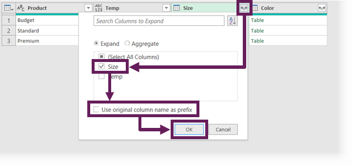
   
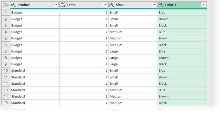
2. The list of possible combinations now appears in the Power Query window.

If you have more than two queries, go ahead and expand those columns too. If you’re working with the example data, the Preview window now looks like this:

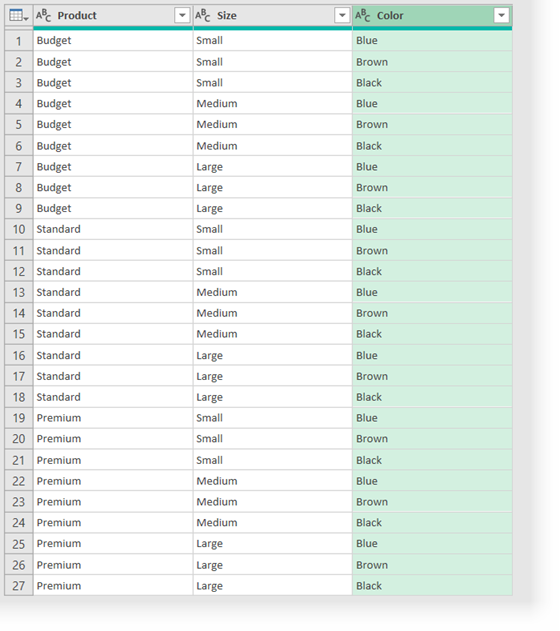
Select the Temp column and press the Delete key as we no longer need this. Finally, rename the columns to be Product, Size and Color.

We now have our list of all possible combinations.

Finally, we just need to load this into Excel, so click File > Close and Load (dropdown) > Close & Load To…

In the Import Data dialog box, select Table and New worksheet, then click OK.

Option #2: Working with tables

There is an easier way, which will be less obvious unless you’ve got a bit of experience of working with tables and lists in Power Query.

Start with the data already loaded into Power Query.

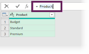
1. From Excel, open a blank query by clicking Data > Get Data > From Other Sources > Blank Query.
2. In the Formula Bar type =Product. (If you’ve not got the Formula Bar open, click View > Formula Bar in the Power Query editor).
   
3. Next, click Add Column > Custom Column
4. In the Custom Column dialog box, enter the following:
   New column name: Size
   Custom column Formula: =Size
   Then click OK.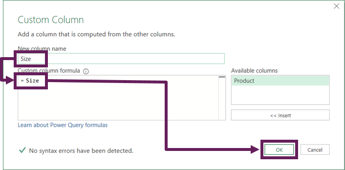
   
5. Add any additional queries in the same way.
6. Expand the tables in the same method as shown in option 1.

This will again give us a table containing all possible combinations.

Now, we just need to load this into Excel. Click File > Close and Load (dropdown) > Close & Load To…

In the Import Data window, select Table and New worksheet, then click OK.

It was a long time after I started using Power Query that I became aware that tables could be used in this way. So hopefully, you’ve learned something new.

Conclusion: List all possible combinations

Getting a table of all possible combinations into Excel may not be as simple as we had wanted. But hopefully, this post has shown that we can achieve it with a few steps.

There is just one warning from me. From 3 lists containing 3 items, we created 27 rows. Now imagine working with hundreds or thousands of rows. That could result in a lot of data. Assuming all the lists are unique, then it follows the basic principles of multiplication. 1000 rows combined with another 1,000 rows would give 1,000,000 rows!!!! So this can become overly cumbersome if we have a lot of data.

Related Posts:

• Introduction to Power Query
• Power Query: Lookup value in another table with merge
• How to combine rows in Power Query

---

What next?

Discover how you can automate your work with our Excel courses and tools.

The Excel Academy