AVERAGE is one of those easy functions in Excel. Like, super easy! It has just one argument, the cells, or numbers to be averaged. So what’s the problem? It’s too easy to get wrong, yet we might not notice for weeks, months, years or ever.
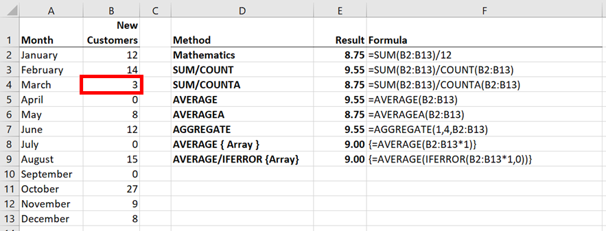
Look at the screenshot below. The result of each method for calculating an average is 9, which is the result we are expecting.
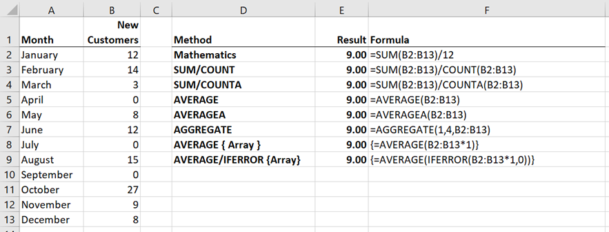
You might be wondering why we need so many methods of calculating an average. As we consider different data scenarios, these formulas will start to show different results.
Most of the formulas are simple enough to understand without explanation, but I will highlight a few of the more unfamiliar:
AVERAGEA or COUNTA functions
These functions include all the populated cells, rather than just the numerical cells.
Array formulas
The formulas with {Array} in their description are special formulas. Enter these by pressing Ctrl + Shift + Enter, which adds curly brackets at the beginning and end. Do not type the curly brackets; Excel will insert them itself.
These formulas perform a calculation on an array of cells before proceeding. Look at the example below:
{=AVERAGE(B2:B13*1)}
Each cell in the Range B2-B13 is multiplied by 1 before it proceeds to be averaged. It is the multiplication of every cell within a single formula which makes it an array formula.
Click here to learn more about array formulas.
AGGREGATE function
The AGGREGATE function includes the ability to calculate an average whilst excluding specific elements, such as errors or hidden rows.
Click here to learn more about the AGGREGATE function.
Now let’s work through some scenarios to show how small changes in data can cause havoc with the results.
Problem #1 – Text included within the dataset
In the screenshot below, the dataset has changed; the text string of “None” has replaced the zero values.
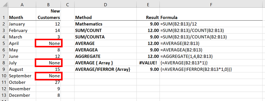
The result of the average formulas now includes a mix of values.
Formulas including COUNT, AVERAGE and AGGREGATE all calculate as 12, rather than 9, as these functions ignore text values. As a result, the total divides by the cells containing numbers, rather than the total number of cells.
COUNTA and AVERAGEA include text cells within the calculation, therefore the calculation result remains at 9.
The AVERAGE { Array } function multiplies each value by 1 before applying the average. Causing an error, as a text string cannot be multiplied by a number.
The AVERAGE IFERROR { Array } formula calculates the correct value of 9. The IFERROR function calculates first, forcing any errors to zero, therefore when the average is applied no text values remain.
Problem #2 – Blank cells included within the dataset
In the screenshot below, the dataset has changed; the zeros from the original example are replaced with blank cells.
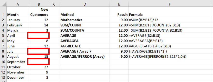
The result of the average formulas includes just two results 9 or 12.
COUNT, COUNTA, AVERAGE, AVERAGEA and AGGREGATE functions all exclude the blank cells in the cell count. Causing these formulas to calculate incorrectly.
The AVERAGE { Array } and AVERAGE IFERROR { Array } formulas multiply the blank cells by 1, which forces them to zero values before calculating the average. The calculation result of these formulas remains correct at 9.
Problem #3 – numbers formatted as text
In this final example, the value in Cell B4 is formatted as text.
There are two potential issues here:
- The total value may exclude the number formatted as text
- The cell count to divide by may exclude the text cell.
COUNT, AVERAGE and AGGREGATE functions exclude the text within the cell count, causing an incorrect total to divide by 11, rather than 12 cells (i.e., both issues have occurred)
COUNTA, AVERAGEA functions will include the text when calculating the cell count, but not in the total. Therefore, the wrong value is divided by the correct number of cells (i.e., the first issue has occurred)
The two { Array } functions calculate the correct value. Any number formatted as text multiplies by 1, converting the text to a number; maintaining the total value and cell count.
Comparison of all formulas
How well did each formula perform across all the scenarios?
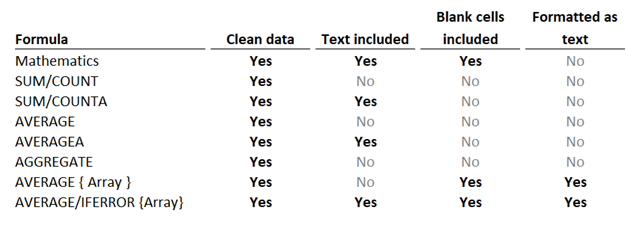
There is only one formula which calculated the correct result across all scenarios, the AVERAGE/IFERROR { array } formula.
It is worth noting that, in this post, I have made a significant assumption. I have assumed we want to calculate the same result as the original data. But what if we want to exclude blank cells or text values? The array function which calculated correctly no longer meets our requirements. We would need to pick another formula.
There is no perfect formula solution for all scenarios as so much depends on user intent.
Conclusion
There are many ways to calculate an average. Different formulas will fit with different datasets and scenarios. The critical thing is to know your data and exactly what you want to achieve.
If you do not have control over the dataset, consider adding a check formula. For example, the ISNUMBER formula will calculate to TRUE if all the cells in the dataset are numbers, otherwise it will calculate to FALSE. Adding the IF function, the formula below would display “Text included in dataset” if any cell in the range B2-B13 were not a number.
=IF(ISNUMBER(B2:B13),AVERAGE(B2:B13),"Text included in dataset")
Related Posts:
How to calculate Weighted Average in Excel
Discover how you can automate your work with our Excel courses and tools.
The Excel Academy

Make working late a thing of the past.
The Excel Academy is Excel training for professionals who want to save time.
The value of mathematical average and AVERAGE function is not identical in EXCEL. While calculating the speed the values by both the methods are different.
why is it so?
how to find the actual value?
I tried the following formulas and I still get #div/0!
=average(e3:e119)
=averageif(e3:e119,”-“)
I need to calculate the average handle time (for calls) and there are rows that show – in the exported data.
Any ideas, why the formulas doesn’t work?
Thanks for your help!
Hi Sima – My guess is that the data in cells E3 to E119 are all text values (or maybe numbers entered as text).
Make sure you don’t have any extra punctuation in the formula – I just spent the better part of an hour trying to figure out my problem before discovering an extra comma in my formula after the last digit and before the closing parentheses.
That’s good advice for all formulas 🙂