From stock parts to holiday villas, from employees to logos, there are plenty of reasons to insert and automatically change an image based on a cell. You may think of this as a lookup function that returns a picture, rather than a value. Ultimately, the purpose is to link an image or picture to a cell; change the cell value and the picture automatically changes.
The Beta version of Office 365 has an IMAGE function that works with web images. That feature has not yet been fully released; Therefore, I believe the methods presented below are best available.
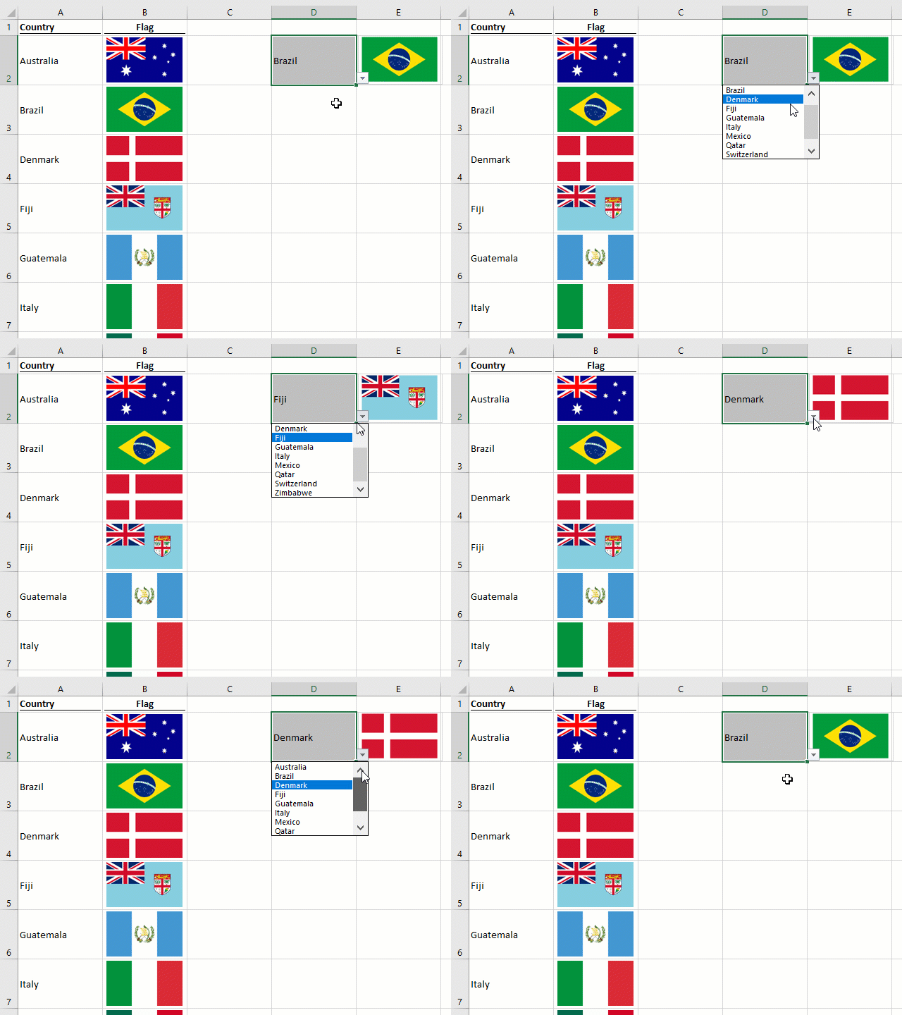
In this post, we’ll explore three different methods to achieve this task. Each solution has it’s own strengths and weaknesses; learn them all and pick the one which best meets your requirements.
Let’s look at each of these methods in turn.
Table of Contents
- Change image with a named range + INDEX/MATCH + linked picture
- Create a dynamic named range with INDEX MATCH
- Using a named range as the source for a linked picture
- The “Reference isn’t valid” Error
- Other formula options
- Change image with chart fill + #N/A
- Formula to calculate as 1 or #N/A
- Create a stacked column chart
- Add the chart fill automatically with a macro
- Change image with a VBA User-Defined Function
- Advantages & disadvantages of each option
- Conclusion
Download the example file: Join the free Insiders Program and gain access to the example file used for this post.
File name: 0004 Change image based on a cell.zip
Change image with a named range + INDEX/MATCH + linked picture
If you’re working along with the example file, we’ll begin with the Linked Picture tab.
As an overview, this method works as follows:
- Create a dynamic named range using the INDEX MATCH formula combination
- Use the named range as the source for a linked picture
Now let’s look at each of these steps in turn.
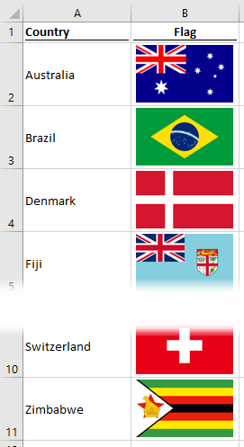
The example data contains a list of countries in Column A and their relevant flags in Column B.
Create a dynamic named range with INDEX MATCH
Start by entering one of the country names in a cell (for our example, use cell D2).
Next, we’ll create a named range by selecting Formulas -> Define Name from the ribbon.

In the New Name dialog box, create a new named range called CountryLookup.
Rather than a range, the Refers to box needs to contain a formula calculates to a range. We will use INDEX/MATCH for our example.
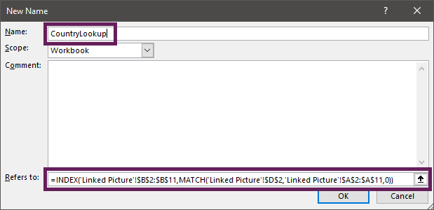
The formula in the Refers to box is:
=INDEX('Linked Picture'!$B$2:$B$11,
MATCH('Linked Picture'!$D$2,'Linked Picture'!$A$2:$A$11,0))
In this formula:
- Cells B2-B11 contain the flags
- Cell D2 contains the name of the country to be matched
- Cells A2-A11 contains the names of the countries
Click OK to close the New Name dialog box.
Using a named range as the source for a linked picture
Now that the named range has been created, follow the following steps to create a linked the picture.
- Select any cell which contains a flag.
- Click Home -> Copy (or Ctrl + C) to copy the cell.
- Select a different cell (use E2 if working with the example file).
- Click Home -> Paste (drop-down) -> Linked Picture (alternatively, the Camera Tool is an option).
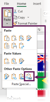
- The pasted image will appear.
- Select the pasted image.
- Change the address in the formula bar to be equal to the named range we created earlier (CountryLookup in our example).
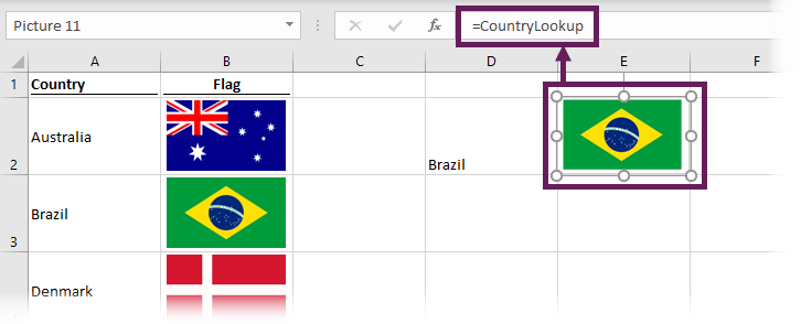
Change the name of the country in cell D2 and watch the image change. For completeness, change cell D2 into a data validation drop-down list containing all the countries.

The “Reference isn’t valid” Error
If you receive the Reference isn’t valid error there are two likely problems:
- The result of the INDEX/MATCH function produces an error. This usually occurs where the name of the country is not identical to one of the countries in the list.
- The named range applied to the picture does not exist.
Other formula options
INDEX/MATCH is a formula combination, which can achieve some amazing things; picture formulas are just one of those amazing things. But any formula which returns a range will work inside the named range. Some easy alternatives are:
XLOOKUP (new function available in Excel 365)
=XLOOKUP('Linked Picture'!$D$2,'Linked Picture'!$A$2:$A$11,
'Linked Picture'!$B$2:$B$11)
Find out more about the XLOOKUP function in this article: XLOOKUP function (support.office.com)
OFFSET / MATCH
=OFFSET('Linked Picture'!$A$1,MATCH('Linked Picture'!$D$2,
'Linked Picture'!$A$2:$A$11,0),1)
To learn about other formulas that return ranges, check out this post.
Change image with chart fill + #N/A
If you’re working along with the example file, check out the Chart Fill tab.
As an overview, this method works as follows:
- Create a formula that calculates 1 for the selected country or #N/A for the other countries.
- Create a stacked column chart with the country list and formula created in 1 above as the source
- Add the images as the fill for each chart series
Here are those steps in more detail
Formula to calculate as 1 or #N/A
Enter a country name in a cell (for our example, use cell D2).
Columns A contains the names of countries.
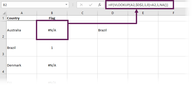
Enter the following formula in cell B2:
=IF(VLOOKUP(A2,$D$2,1,0)=A2,1,NA())
The purpose of the formula is to calculate 1 if cell D2 is the same as the country in column A; otherwise, #N/A is displayed. Copy the formula down to the last country name in the list.
Create a stacked column chart
Now it’s time for the chart trickery:
- Select the list of country names and the formula result (cells A2 to B11 in our example).
- From the ribbon, click Insert -> Charts -> Stacked Column

- A new chart will appear on the worksheet.
- Right-click on the series, then click Select Data… from the menu.
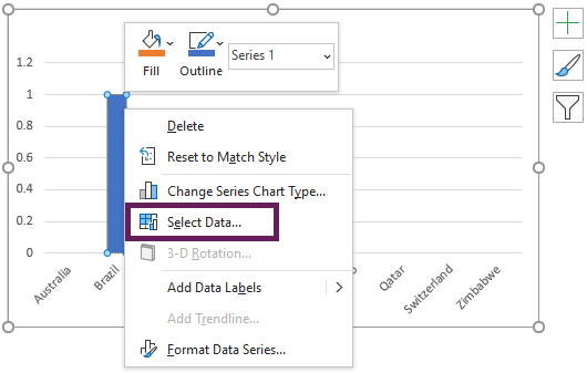
- The Select Data Source dialog box will open.
- Click the Switch Row/Column button, the Legend Entries box on the left should now contain the list of countries as different chart series.
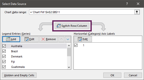
- Click OK to close the Select Data Source dialog box.
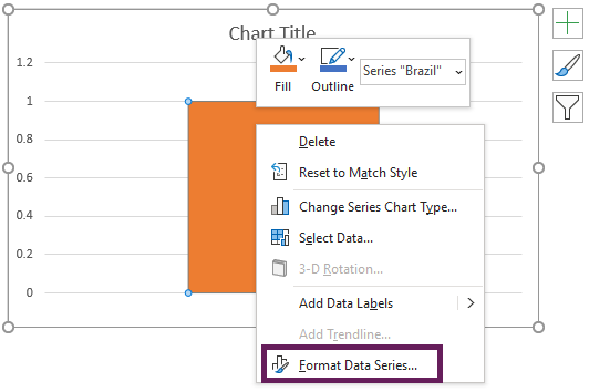
- Right-click on the data bar and select Format Data Series… from the menu.
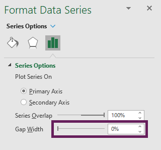
- Change the Gap Width to 0%
- Right-click on the vertical axis and select Format Axis… from the menu.
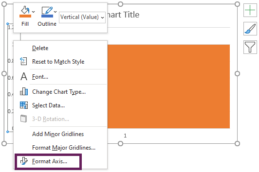
- Set the axis maximum equal to 1.
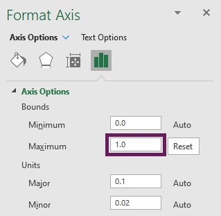
- Select the Chart Title, press the delete key.
- Next, select the vertical axis and delete it.
- Then, select the horizontal axis and delete that also.
- Re-position and resize the chart to fit your requirements. The worksheet will look similar to this:

- Change the selected country to be the first country in the list.
- Right-click on the chart fill and select Format Data Series… from the menu.
- Change the fill to Picture or texture fill and click Insert…
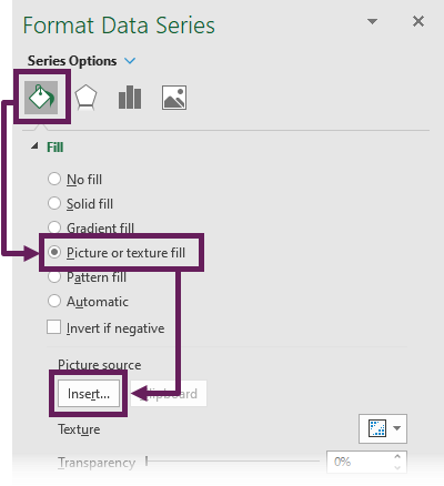
- Navigate to the picture location and click Insert.
- Repeat steps 16 to 19 for each country in the list.
The fully working chart achieves a similar result to the first example.
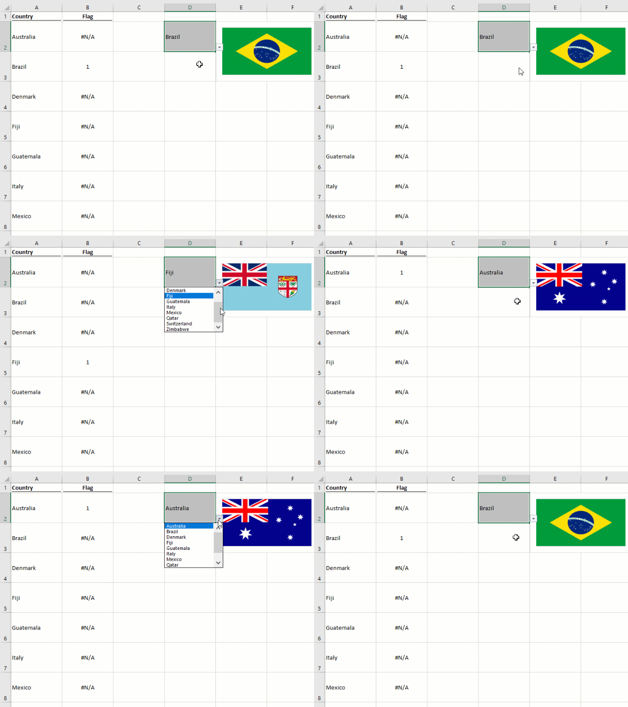
Inserting images one at a time, in this way, can be time-consuming. So, I have created a macro that can automate this for you.
Add the chart fill automatically with a macro
The macro below inserts pictures into the chart fill automatically. To work, the names of the countries must exactly match the names of the pictures.
To run the macro for your scenario:
- Change “Chart 1” to the name of your chart.
- Set the file path to the folder containing the images, and change the file extension.
- In the worksheet, select the cells containing the country names and run the macro. The chart should automatically populate with the relevant images.
Sub InsertPicturesIntoChart()

Dim i As Integer
Dim selectedCells As Range
Dim imageFullName As String

'Select the cells with the country names before running macro
For Each selectedCells In Selection

    i = i + 1

    'imageFullName is the file path to the image.
    'Country name in Column A must match the name of the image.
    imageFullName = "C:\Users\marks\Documents\Flags\" & Cells(i + 1, 1).Value & ".png"

    'Change the fill of the chart Series. Change Chart 1 to the name of the chart.
    ActiveSheet.ChartObjects("Chart 1").Chart.SeriesCollection(i).Format.Fill.UserPicture imageFullName

Next selectedCells

End Sub
Change image with a VBA User-Defined Function
If you’re working along with the example file, look at the UDF tab. Finally, we will consider a VBA user-defined function. This is a formula created using VBA macros to insert and change pictures. Learn more about UDF’s here.
WARNING! User Defined Functions that change objects are not officially supported in Excel. While this works in the Windows version of Excel, I’ve not successfully made it work on the Mac version. Other VBA options are available, but they are not as flexible as the UDF method presented here.
The VBA code
Copy the following code into a standard module within the Visual Basic Editor.
Public Function PictureLookupUDF(FilePath As String, Location As Range, Index As Integer)

Dim lookupPicture As Shape
Dim sheetName As String
Dim pictureName As String

pictureName = "PictureLookupUDF"

sheetName = Location.Parent.Name

'Delete current picture with the same Index if exists
For Each lookupPicture In Sheets(sheetName).Shapes
    If lookupPicture.Name = pictureName & Index Then
        lookupPicture.Delete
    End If
Next lookupPicture

'Add the picture in the right location
Set lookupPicture = Sheets(sheetName).Shapes.AddPicture _
(FilePath, msoFalse, msoTrue, Location.Left, Location.Top, -1, -1)

'Resize picture to best fit the range
If Location.Width / Location.Height > lookupPicture.Width / lookupPicture.Height Then
    lookupPicture.Height = Location.Height
Else
    lookupPicture.Width = Location.Width
End If

'change the picture name
lookupPicture.Name = pictureName & Index

PictureLookupUDF = "Picture Lookup: " & lookupPicture.Name

End Function
Using the UDF on the worksheet
The user defined function can now be used on the worksheet just like a normal function.
The PictureLookupUDF uses the following arguments:
=PictureLookupUDF(FilePath, Location, Index)
- FilePath = Full file path to the image, including the file extension.
- Location = Range of cells where the image should be placed.
- Index = A unique reference number to identify the image.
The formula is used in the example below.
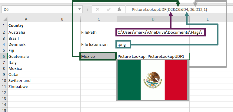
In cell D6 the formula is:
=PictureLookupUDF(D2&C6&D4,D6:D12,1)
- D2&C6&D4 – consolidates the folder path, country name, and file extension
- D6:D12 – the range of cells of where the place the picture
- 1 – the unique reference number to identify the image
WARNING! – Make sure the folder path contains a slash before the file name.
Images can be placed on a different worksheet, by using a standard sheet reference:
'Sheet 1'!$D$6:$D$12
Look at this function in action. It behaves just like the previous examples.
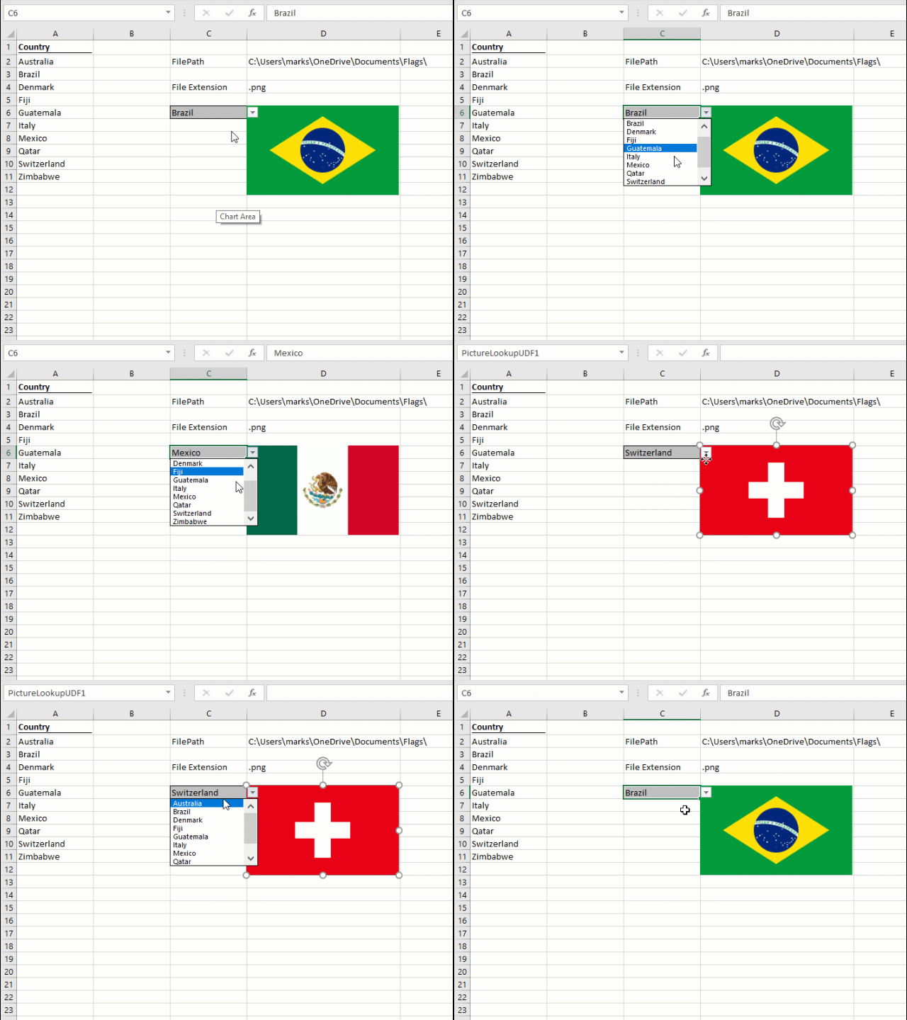
The Index argument can be used to insert multiple images. For example, to include a second image, increase the index number by 1, as shown below.
=PictureLookupUDF(D2&C16&D4,D17:D23,2)
If you wish to amend the VBA code to change the images further, such as size, rotation, etc., you can find further guidance here.
Advantages & disadvantages of each option
Named range + INDEX/MATCH + linked picture
Advantages:
- All the images are contained on the worksheet
Disadvantages:
- Could accidentally move images outside of the cell range
- Takes a lot of preparation to use multiple images
Chart fill + #N/A
Advantages:
- Images contained within the chart, so difficult to change images in error
Disadvantages:
- Time-consuming to set-up
- Requires a helper column to function correctly
- Takes a lot of preparation to use multiple images
VBA User Defined Function
Advantages:
- No additional columns required on the worksheet
- Easy to use with multiple images
Disadvantages:
- Technique not fully supported by Microsoft
- Requires users ability to use VBA
- Image name must be the same as the value on the worksheet
- Difficult to share the workbook with others who don’t have access to the image folder
Conclusion
There are many ways to change an image based on a cell value. Only one VBA option has been presented in this post, but there are many other possible solutions.
Which method should you use? It really depends on your circumstances. My advice is to learn them all and apply what you think works best in each scenario.
Discover how you can automate your work with our Excel courses and tools.
The Excel Academy

Make working late a thing of the past.
The Excel Academy is Excel training for professionals who want to save time.

Hi! Awesome functions, I got finally my template to work as intended. But I do have still one issue:
What if I would need the function “Index/Match” to perform it’s action (meaning “fetch the picture to cell E2” in your example sheet) ONLY IF there is a country added into the cell D2? What I mean is that IF cell D2 is empty, the function “shouldn’t do anything” in cell E2?
Now I basically have solved this issue with extra value on the Linked Picture list saying “No country” and then I added as the flag pic just an empty white box. So if you choose “No country” in cell D2, it fetches the white box into cell E2. I am fine with this but there is a risk if someone decides to use some other colored paper than white so I am already seeing the complaints that what are the boxes 🙂
Thank you so much already in advance if you’re able to help me here!
Hi Johanna,
You could try wrapping the INDEX/MATCH function in an IFERROR function. I think IFERROR was introduced in Excel 2007, so should be safe to use now.
Using the example file, the formula would be as follows:
=IFERROR(INDEX('Linked Picture'!$B$2:$B$11,MATCH('Linked Picture'!$D$2,'Linked Picture'!$A$2:$A$11,0)),'Linked Picture'!$C$2)The last reference of ‘Linked Picture’!$C$2, just has to refer to any blank cell.
It should work because, if a lookup is not found a #N/A error is returned by the INDEX/MATCH, this will trigger the IFERROR and point to Cell C2. Hopefully that makes sense.
Hopefully that helps.
Thanks,
Mark
Hi all,
I tried this function on a protected sheet but it didn’t work even if added a code to unprotect the sheet at the beginning of the function (UnprotectSheet Sheets(“Sheet1”)).
Is there a way to fix this issue .
Thanks.
Unfortunately not. UDF’s don’t mix well with protected sheets… sorry.
The other methods appear to work OK on protected sheets.
Hi,
Thank you for this code… its Awesome!
How do I go about if I want to insert the image to the center of the selected range of cells and not to the Left Top?
Thanks!
You just need the width and height of both the image and the range of cells.
As an example, to put an image in the centre of cell B2 – H8 you would use:
ActiveSheet.Shapes("myPic").Left = ActiveSheet.Range("B2").Left + _ ActiveSheet.Range("B2:H8").Width / 2 - _ ActiveSheet.Shapes("myPic").Width / 2 ActiveSheet.Shapes("myPic").Top = ActiveSheet.Range("B2").Top + _ ActiveSheet.Range("B2:H8").Height / 2 - _ ActiveSheet.Shapes("myPic").Height / 2hi there,
Thanks so much for your helpful description and files.
Just a small comment concerning the VBA-chapter. I experienced some issues using commas instead of semicolons when separating the values in the formula.
You wrote the following code:
=PictureLookupUDF(D2&C6&D4,D6:D12,1)
Shouldn’t it be this instead:
=PictureLookupUDF(D2&C6&D4;D6:D12;1)
The use of commas or semi-colons is dependant on your regional/language settings in Excel. Use the argument separator you would normally use for standard functions.
the picturelookupUDF works great, but i have one problem. the unique identifier. Is there a way to have it change on its own? IE: when i copy the following formula “=PictureLookupUDF($E$2&A2&$E$3,B2,1)” 1 cell down, i would like it to change to “=PictureLookupUDF($E$2&A3&$E$3,B3,2)”
Use the ROW() function to calculate the number.
e.g.
ROW(A2) – ROW($A$1)
is there a way of doing this on Excel Online? (Ultimately the sheet will be embedded in a webpage so need this to happen on Excel Online).
There isn’t a way to do this with VBA. Excel Online uses Office Scripts, which has only recently been released. I don’t know whether it is possible to do this with Office Scripts or not. You may be the first person to try.
Is there a way to do this for a whole table, in which a single picture (indexed from a table of five picture options) appears per row based on the immediate cell value on the left of each row (previous column), which is generated by a conditional fromula (it is changing). Or do I have to do the whole table (100 values one by one)?
If you use the UDF method it should be possible to use a table. You’ll need to change the picture index number to ensure it is unique (you could use the ROWS function to create that).
All the other methods will involve creating the objects individually. Unless you write a macro which can create these for you.
As the UDF method is not officially supported by Microsoft, it may not be compatible with other things you want to do, such as protecting the worksheet.
Any use of images will be slow for Excel to calculate. So if using 100 images, recalculation times will be affected.
Thank you very much!!! Quite smart trickies!
Hello , This is exciting pproject .
I need your help about my requirment #.
I want to kinow how we can extend this formula to other rows of column D to be general for all rows of D column .
I mean I need when in D3 cell, a country is selected , the flag of that country would be shown in E3 . in D4 , the flag of appropirated country in E4 and D1000 could shows the flag in E1000 , etc …
I need this for a table ( recordset ) in a dataset .
Thanks in advance
Mehdi
Check out the section entitled: Change image with a VBA User-Defined Function. That method allows lots of images to be used. But if you’re using 1000 rows, it’s going to be excessively slow.
Hello – does the VBA User-Defined Function approach work on Macs? I am trying in now and it doesn’t seem to be working.
I’ve never tried it on a Mac. The compatibility between Windows and Mac isn’t great, and it even changes across different Mac versions. So it wouldn’t surprise me if it doesn’t.
I used the 3th option(VBA). First it was working well, but suddenly the position of my picture is placed 2 row below. If I change the size / position of cells, it keep staying 2 cells below my upper cell selection. If I try it again in another excel file, it work well.
What should be the problem the position of my picture is still below my upper selection?
Thank you!
Hi,
I published a message one week ago. Everything is working but the pictures are not always no the same place. I am using the VBA method. Now as example… I have the PictureLookup code in cell C3. My first cell I need to select is the cell where the information will be. Like in your situation, Brazil/Italy/… . I put this in A3. If I refresh cell A3 with Brazil, my picture is going up or down. If I refresh C3 where the code is, the pictures is going back on the right position. The bizar thing is, If I am working with 2 screens, and I put my excel on the second screen, the position when refreshing A3(brazil/Italy) is different then with my main screen. Also with refreshing C3. What is the problem here? Is there a possibility to put an extra line vba code with every refreshing, he also refresh the C3 code or the cell where the Picture Lookup is put in?
Thank you very much
Hi Gianni – hmmm an interesting problem. Is it always a consistent distance from the cell?
I wonder if your screen are at different pixel rates, therefore Excel is doing the calculation in one instance of Excel, but rendering the result in another.
Without seeing the issue, it’s difficult to comment.
Hi it works well however the picture has a border, how do I remove it?
Which method of you used? The process to remove the border will be different for each of them.
I am using the INDEX MATCH way.
Every time I paste the image using “Linked Picture”, it pastes as a AutoShape object instead of a Picture.
Because it pastes as an AutoShape and not a Picture, It will return text or number values IN the cell but not the picture data on top of the cell.
Do you have any ideas on how to fix this?
I’ve not had the specific issue you’re running into. Are you using the right kind of image paste?
Hi, Nice tutorial!!!
Now tried to expand on this using version 1.
My snippit looks like(platform in german):
=INDEX(INDIREKT(ADRESSE(2;3;;;”Branding”)&”:”&ADRESSE(((ANZAHL2(Branding!B:B)-1)*2);3));VERGLEICH(Branding!$J$1;INDIREKT(ADRESSE(2;2;;”Branding”)&”:”&ADRESSE(((ANZAHL2(Branding!B:B)-1)*2);2));0))
It’s just I’m not getting further?
Respects
Hames
This doesn’t work properly on Macs running Excel 2016. Only a portion of the flag is visible when the country is selected from the pull-down menu. Any thoughts on how to fix this? I can see lots of applications for this if I can get this to work.
Windows and Mac versions of Excel just aren’t as comparable as Microsoft may try to make us believe. I suspect it’s either a bug, or not supported in the Mac version.
Super nice VBA, works right off as expected!
Is there an easy way to remove the error message box if the filename (C6) is empty? I’m trying to work with multiple instances (10ish) of the formula and they would be used as an empty template. The problem is I keep getting all the empty cells errors boxes everytime.
Thanks!
It would simply work with a if-statement. Its more simple than index, or match.
It havent worked for me.
It could work with IF. It would work with any function that returns a range. Change out this post for examples: https://exceloffthegrid.com/cell-ranges-basic-things-99-users-dont-know/
If you have a lot of images, IF would be very hard to manage. While INDEX/MATCH can easily handle large ranges.