We have all experienced it, and often at the worst possible moment. For whatever reason, Excel’s formulas aren’t calculating correctly. The good news is that it is usually something simple. Once we know the most likely causes, it is easier to troubleshoot the problem. So, in this post, we look at the most likely reasons for Excel formulas not calculating.
The 14 reasons and fixes in this post, should give you what you need to know. So, if you’re concerned that Excel has stopped calculating or that numbers aren’t updating, we have the answer for you.
Table of Contents
- Calculation option – automatic or manual (#1)
- Wrong number format (#2)
- Leading apostrophe (#3)
- Leading and trailing spaces (#4)
- Numbers contained in double quotes (#5)
- Incorrect formula arguments (#6)
- Non-printed characters (#7)
- Circular references (#8)
- Show formulas (#9)
- Incorrect cell references (#10)
- Automatic data entry conversion (#11)
- Leading Zeros (#12)
- Hidden rows and columns (#13)
- Binary to decimal conversion (#14)
- Conclusion
Watch the video

Calculation option – automatic or manual (#1)
Excel has two calculation options, Automatic and Manual. Most users don’t even know these two modes exist. Yet, frustratingly, in some circumstances, they can change without us knowing it.
Automatic calculation is the default mode. This is where formulas recalculate after any change affecting the result of a calculation.
Excel formulas are efficient at handling calculations. In the background, Excel knows which cells impact which formulas. Therefore, the Automatic calculation mode recalculates the minimum number of cells. This ensures Excel is fast while keeping all the values up-to-date. This is the behavior that we understand and expect.
However, due to the size and complexity of some spreadsheets or due to 3rd party add-ins, calculation speed can become very slow. This leads some users to change Excel’s option to Manual calculation mode. Consequently, Excel doesn’t recalculate anything. In Manual calculation mode, we can change cell values, but nothing happens. Therefore, we must explicitly tell Excel when to recalculate.
Therefore, if Excel is in manual calculation mode, it would appear there is an issue because we see Excel formulas not calculating.
NOTE: Unfortunately, Excel can change between Manual and Automatic calculation modes without us knowing it. So check out this post: Why does Excel’s calculation mode keep changing?
To determine which calculation mode is enabled, click Formulas > Calculation Options (drop-down). The tick inside the drop-down identifies which calculation option is applied.
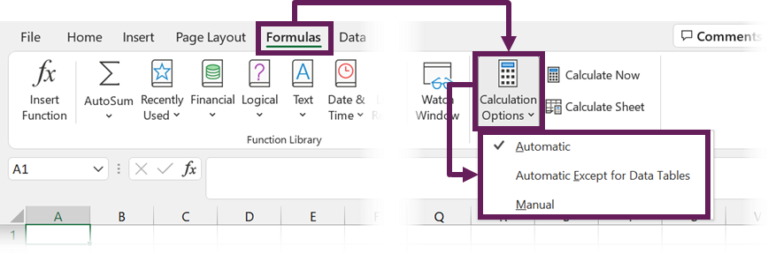
Click Automatic to ensure the calculation happens automatically.
Calculation mode is an application-level setting; therefore, it applies to all open workbooks.
If you want to remain in Manual calculation mode, here are some useful shortcuts.
- F9: Calculates formulas that have changed since the last calculation, and formulas dependent on them, in all open workbooks.
- Shift + F9: Calculates formulas that have changed since the last calculation, and formulas dependent on them, in the active worksheet.
- Ctrl + Alt + F9: Calculates all formulas in all open workbooks, regardless of whether they have changed since the last time or not.
- Ctrl + Shift + Alt + F9: Rechecks dependent formulas and then calculates all formulas in all open workbooks, regardless of whether they have changed since the last time or not.
This is probably the #1 reason why we see Excel formulas not calculating.
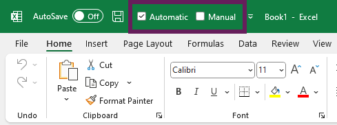
TOP TIP: Add the Automatic/Manual calculation options to your QAT. This is an easy way to switch between modes and identify which mode is active.
Wrong number format (#2)
When looking at cell values, we decide what kind of data it is. We know instinctively that numbers can be aggregated, but text cannot. Unfortunately, Excel isn’t so clever.
Within Home > Number, we can select the cell format.
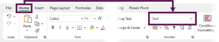
If a cell is formatted as text instead of a number, Excel may not calculate and may not display the value we expect.
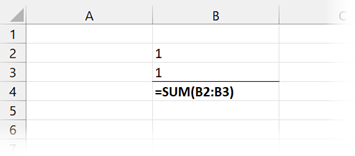
Look at the screenshot below.
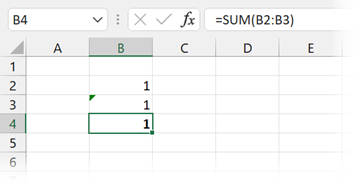
In Cell B4, the SUM of B2:B3 equals 1; 1+1 = 1 is definitely wrong. This is because B3 is formatted as text, and the SUM function ignores text. So, while the calculation may look like 1+1 = 1 (which is wrong), it is actually 1+0 = 1 (which is correct).
To fix this, here are 3 options:
- Manual change
- Change the cell format from Text to another format (General is a good option to start with)
- Double-click on the problem cell to go into edit mode
- Press return to commit the formula
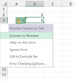
- If the cell has a green triangle:
- Click on the cell
- Select Convert to number from the warning drop-down
- Adding zero to the number
- Select any blank cell.
- Copy the cell
- Select the cells to be converted to numbers
- Click Home > Paste > Paste Special…
- In the Paste Special window, select Add, then click OK
#1 specifically relates to numbers formatted as text, but #2 and #3 can be used in many scenarios where numbers are stored as text.
Leading apostrophe (#3)
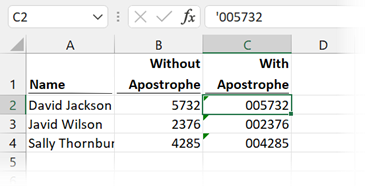
The apostrophe ( ‘ ) is a special character in Excel. Whenever an apostrophe is entered at the start of a value or formula, this tells Excel that everything that follows is text.
This special character ensures we can store numbers as text. For example, if we wanted to hold an employee number containing leading zeros, Excel might remove the zeros on data entry.
Therefore, we insert the apostrophe to ensure Excel understands this as text.
However, sometimes an apostrophe can appear when we don’t want it. This often happens when the data is imported from an external system.
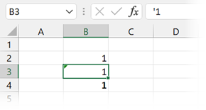
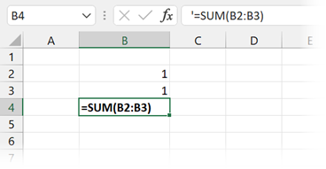
The screenshot below shows a calculation that doesn’t work as expected. The formula in Cell B4 is SUM(B2:B3), therefore 1 + 1 = 2, yet the value in B4 equals 1. This is because cell B3 contains a value with an apostrophe preceding it.
Either remove the apostrophe manually or use techniques #2 and #3 listed in the section above to fix the issue.
There is a similar impact on formulas. For example, in the screenshot below, the SUM function has a leading apostrophe; therefore, it is treated as text.
As it’s a formula, you will need to remove the apostrophe manually. Then you’re good to go.
Leading and trailing spaces (#4)
Leading and trailing spaces are a big problem, they often occur in imported text, but we cannot see them with our eyes.
Let’s look at an example.
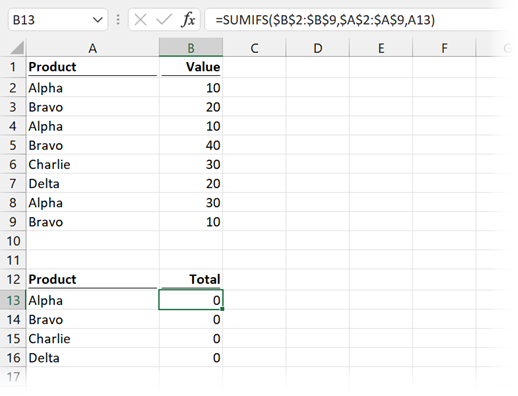
In the screenshot above, the formula in Cell B13 is:
=SUMIFS($B$2:$B$9,$A$2:$A$9,A13)We are performing a basic SUMIFS function to add the values for product Alpha. Based on the data, the value should be 50, but it calculates as zero.
The problem is that all the values in Cells A2:A9 have trailing spaces. Rather than “Alpha”, used in Cell A13 for the SUMIFS function, the value in the data is “Alpha “ (with trailing spaces). Excel views these as different values. As a result, there is no match.
To fix this, there are lots of options. Some suggestions are:
- Manually removing the space from the data
- Adding the trailing space into our SUMIFS criteria
- Using the TRIM function to remove extra spaces from the start/end of the text
- If there are no spaces in the middle of the text, we can use Find and Replace to remove extra spaces.
Numbers contained in double quotes (#5)
Another text/number mix-up issue occurs when numbers are included in double-quotes.
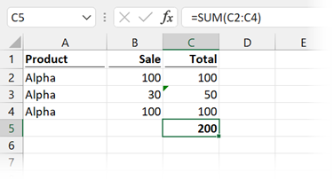
Look at the screenshot below. There is a problem; 100+50+100 definitely does not equal 200.
In this scenario, there is a minimum sale volume of 50; therefore, using an IF function, the value in row 3 has increased correctly from 30 to 50. Consequently, the total should be 250. So, what’s happened?
The problem is due to the calculation in Cell C3.
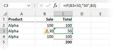
The formula is:
=IF(B3<50,"50",B3)In Cell B3, the value is less than 50; therefore, the text value of “50” is returned in Cell C3. The double quotes tell Excel that this is text and not a number.
To fix this, remove the double quotes around the number 50. Then the correct total will be calculated.
Incorrect formula arguments (#6)
Excel functions are a programming language for calculating a result. Each function has its own syntax (i.e., the arguments required to calculate an outcome). If we get this syntax wrong, it can lead to unexpected results.
VLOOKUP is a very error-prone function; it has caught out many unsuspecting users.
Let’s take a look at an example.
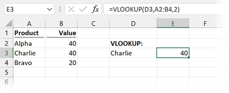
In the example above, the formula in Cell E3 is:
=VLOOKUP(D3,A2:B4,2)It results 40 for Charlie, which is correct.
Now let’s change the value in D3 to Bravo:
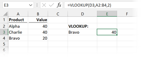
It still returns 40!! Bravo should be 20. How is that possible?
In our formula, we excluded VLOOKUP’s 4th argument, which is the Range_Lookup argument.
- If we enter TRUE or exclude this argument, we are telling Excel that :
- the first column in our data is in sorted ascending order
- we want to return the value closest to, but not greater, than the lookup value (known as an approximate match).
- If we enter FALSE as the fourth argument, Excel only returns an exact match.
Our first column is not in ascending order, but by excluding the 4th argument, Excel believes it is sorted. Therefore, Excel calculated the wrong result.
If we go back and change our formula, so the 4th argument is FALSE, it works.
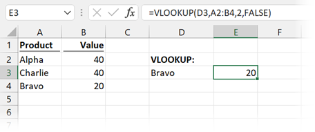
This demonstrates the importance of understanding what all function arguments do.
Non-printed characters (#7)
Non-printed characters are letters used within computer code that a person cannot view. As a simple example, the line break character we can enter into Excel using Alt + Enter is not printable.
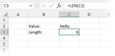
In the screenshot above, the LEN function shows 6 characters in Cell C2. But the word “Hello” only has 5 characters.
There are no spaces in Cell C2, so what’s going on? It’s because there is a trailing line break character.
We can remove non-printed characters using the CLEAN function.
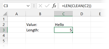
Look at the screenshot above. Once we’ve used the CLEAN function, the value is now correct again.
Circular references (#8)
Circular references are where a formula refers to a cell within its own calculation chain. Here is an example.
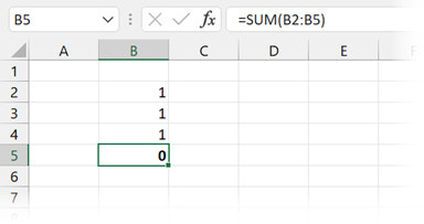
The formula in Cell B5 is:
=SUM(B2:B5)If you notice, the cell reference of the formula (B5) is included within the range of cells (B2:B5). Consequently, Excel cannot calculate a result (unless iterative calculations have been enabled).
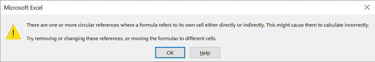
When we create or open a workbook with circular references, Excel will often display an error message:
“There are one or more circular references where a formula refers to its own cell either directly or indirectly. This might cause them to calculate incorrectly.
Try removing or changing these references, or moving the formulas to different cells.“
But, error messages don’t stop us from clicking OK and continuing as if nothing is wrong.
If there are circular references, they can be tough to find manually. Thankfully, Excel has given us a tool within the Formulas > Formula Auditing > Error Checking > Circular References which displays the circular references in any of our open workbooks.
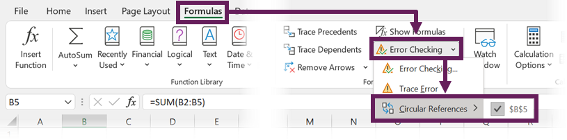
As shown in the screenshot above, Cell B5 has a circular reference. Once we remove that, it will calculate correctly.
Show formulas (#9)
In Excel, we usually view the results of calculations. However, with one mouse click or one shortcut, we can quickly toggle to show formulas rather than results.
Turning on show formulas can easily be performed by accident or saved in this state by a previous user.
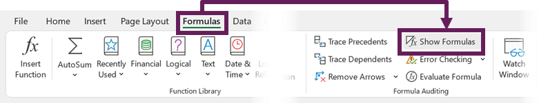
To display the formula results again, click Formulas > Formula Auditing> Show Formulas, or use the shortcut key Ctrl + ` (the key to the left of the 1 key on a standard windows keyboard).
Incorrect cell references (#10)
One thing we learn in Excel quite early on is the use of the dollar ($) symbol to lock cell references. For example:
- If we enter =A1 into a cell and copy it down, it will change to =A2.
- If we enter =A$1 and copy the cell down, it will remain as =A$1.
We get used to this referencing syntax quickly. However, this makes it easy to make mistakes when copying formulas to other cells.
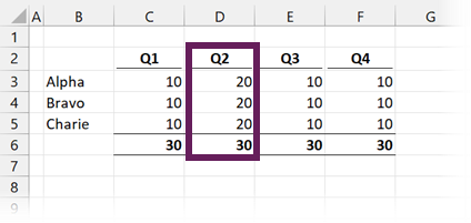
Look at the screenshot above. There is definitely an issue with the calculation in Cell D6.
Double-click on the cell, and the problem will quickly reveal itself.
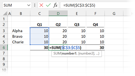
Yes… somebody forgot that $ symbols had been used in the formula in Cell C6, then they copied the formula into Cells D6 to F6.
Unfortunately, it’s easily done; I’ve done it myself many times.
How can we find these types of errors? The only way is to check our work as we go, and apply a healthy bit of skepticism to any calculation result. It’s better to self-review and find an error than to sit in a meeting with your manager, and them find it.
Automatic data entry conversion (#11)
To help reduce the number of errors we make, Excel is programmed to auto-correct / auto-change some data as we enter it. This is great most of the time, and who knows how often it has saved us from an embarrassing mistake.
However, auto-correction can cause problems at other times. For example, what do we want if we enter 1/1 into Excel? Do we want the result of 1? Or do we want 1st January? In this case, Excel assumes we want 1st January of the current year.
Dates are the most common type of automatic conversion. Dates in Excel are actually numbers, based on the number of days since 31st December 1899. So, assuming the current year is 2022, if we enter 1/1, Excel thinks we want 1st January 2022 (which is the number 44562). We can see this when we change the date to a number format.
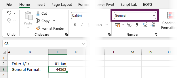
We tried to enter a value of 1/1 and ended up with a value of 44562. Hmmm… that could cause us an issue.
Leading Zeros (#12)
We have already seen above in #3 that leading zeros can be a problem.
If we try to enter a number with leading zeros, such as 0005321, Excel assumes we don’t want the leading zeros and converts the number to 5321.
To retain leading zeros, we should either:
- Add an apostrophe at the start
- Convert the data type to text before entering value
Hidden rows and columns (#13)
This is one of my pet peeves. Hidden rows and columns cause so many problems for Excel users. In my opinion, they should be avoided at all costs.
Let’s look at an example:
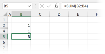
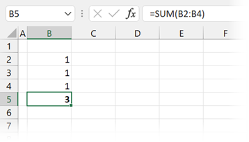
Look at the screenshot above. The formula in Cell B5 is:
=SUM(B2:B4)Is this result correct? Actually, Yes. But the hidden row make the result look wrong. This is because the hidden row contains an additional value, as we can see when we unhide row 3.
If we want a calculation that excludes hidden cells, we should consider using the AGGREGATE or SUBTOTAL function.
Binary to decimal conversion (#14)
Computers store numbers using binary (a mixture of 1 and 0’s). Yet we learn numbers using a decimal base 10 system. As a result, Excel must convert between binary and decimal numbers, which can lead to some unexpected differences.
We know one-third (1/3) cannot be expressed as a decimal; it calculates as 0.333333… recurring into infinity. So we tend to use an approximation with a reduced number of digits.
In binary, there are also numbers that have a recurring number into infinity. One-tenth (1/10) can easily be expressed as a decimal: 0.1. But in binary, it is 00011001100110011… recurring into infinity.
Excel calculates to 15 significant digits. Therefore, it is possible for minor rounding differences to occur due to the conversion from binary to decimal. While this may be insignificant, if this is used in a logic statement, it can lead to an alternative result.
Check out this post for more details: Excel can calculate the wrong results: WARNING
Conclusion
In this post we have given you the most likely reasons we find Excel formulas not calculating as expected. I trust these 14 techniques have helped to solve your problem.
If you’ve found any other simple issues which cause incorrect calculations, please add them in the comments below.
Related posts:
Discover how you can automate your work with our Excel courses and tools.
The Excel Academy

Make working late a thing of the past.
The Excel Academy is Excel training for professionals who want to save time.
The first solution here fixed my exact problem, thanks! had no idea the automatic/manual calculation was a thing.
Great news 👍
I put =NOW() in cell A1 on a new blank sheet. It refuses to update unless I physically double click on it. I toggled Calculation from Automatic to Automatic except tables.
It refuses to update. What can I do Nick? Contact: Ed Davis [email protected]
It is not a live clock. NOW() only updates when the formulas re-calculate.
If you want to show a live clock, you’ll need to include VBA to force the formula to recalculate a 1 second interval