Excel can calculate the wrong results: WARNING

The old proverb is that “a bad workman blames his tools”. As Excel is such a popular tool, it gets a lot of blame when the person using it is actually at fault. However, it is not always a person who is to blame; Excel can calculate the wrong results all by itself!

In this post, I want to explain the cause of the problem and provide methods to avoid it.

Table of Contents

• Spreadsheet errors
• Scenario
• Why does this issue occur?
• Why don’t they fix the problem?
• How can we avoid the problem?
• Using the ROUND function
• Applying precision as displayed
• Wrap-up

Watch the video

Watch the video on YouTube.

Spreadsheet errors

The much-quoted statistic is that 80% of spreadsheets contain errors; therefore, it is not uncommon to find an error in an Excel workbook. The errors referred to in this statistic are all caused by humans. Let’s face it, spreadsheets are complex. They are small applications that do not get the rigorous testing they deserve. Therefore, we should expect errors.

Errors tend to fall into 3 groups:

• Logic errors – caused by the individual not fully understanding the situation and therefore choosing the wrong formula or solution
• Omission errors – caused by cells and ranges accidentally excluded from formulas
• Mechanical errors – caused by data inaccuracy or input/typing errors

There is one other error type – the error where Excel doesn’t calculate the correct numbers.

Scenario

Let’s use a basic scenario. Look at the screenshot below:

The formula in Cell F7 is:

=VLOOKUP(F5,B5:C7,2,FALSE)

This is a basic VLOOKUP function. The formula looks up at the value 20.4 in Cells B5:B7 and returns the corresponding value from Cells C5:C7.

The value returned is Bravo, which is correct.

Now take a look at the second screenshot.

It appears to be exactly the same. Same lookup value, same data, same formula. But, a different result in Cell F7. The value returned is the error #N/A.

The second example proves that Excel can calculate the wrong result!

The only difference between the two scenarios is in Cells B5:B7. In the first screenshot, the values are all hardcoded:

• B5: 20.3
• B6: 20.4
• B7: 20.5

In the second screenshot, the values are calculated:

• B5: 20.3
• B6: =B5+0.1
• B7: =B6+0.1

This is not an issue with VLOOKUP; the same problem occurs with INDEX/MATCH and XLOOKUP.

In this scenario, we have used VLOOKUP with an exact match; therefore, it returns the #N/A error. However, with an approximate match, it would not have produced an error, but the result “Alpha”. Therefore, the impact of this could be hidden and significant in some scenarios.

Why does this issue occur?

Why does Excel have this issue of calculating different results for the same calculation?

We are taught at school that some numbers cannot be expressed as decimals. For example, one-third (1/3) cannot be expressed as a decimal; it is 0.3333… recurring into infinity. So, instead, we might use 0.33 as a close estimate. We fully accept that 0.33 does not equal 1/3 but deem it insignificant.

Computers calculate numbers using binary. In the background, a conversion takes place to change binary to decimal so that we humans can understand it. As you can see below, it is easier to understand a decimal than a binary number.

Decimal: 237 = Binary: 11101101

Every whole number can be converted from binary perfectly. But this isn’t true for every decimal floating point number.

Taking an example, one-tenth (1/10) is easily expressed as a decimal: 0.1. But. 0.1 in binary is 000110011001100110011… recurring into infinity. Just as we cannot correctly write one-third in decimals, one-tenth cannot be stored in binary.

Computers have a finite amount of storage; therefore, they cannot store an infinite number. In addition, Excel is programmed to calculate accuracy to 15 digits of precision. As a result, Excel can never calculate 0.1 perfectly.

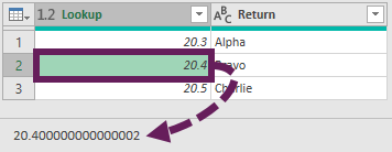
Heading back to our example, if we loaded cells B5:B7 into Power Query, it shows us the underlying number.

20.3 + 0.1 is not exactly 20.4, but calculated as 20.400000000000002.

But wait, take a few seconds to count those digits. The screenshot shows it’s not 15 digits of precision, as Microsoft claims in their specifications documents, but the number is 17 digits long.

OK, let’s try something else. Look at the screenshot below.

The formulas in each cell are as follows:

• Cell B1: 20.4
• Cell C2: =20.3+0.1
• Cell D2: B2=C2

We’ve seen that 20.3+0.1 = 20.400000000000002.

Therefore, the result in D2 should be FALSE. The VLOOKUP result above tells us that these two are not the same. Yet, the result in D2 is TRUE.

We can conclude from this that some Excel functions calculate using 15 digits of precision while others use 17.

NOTE: 0.1 is not the only number to have this issue, but it is the easiest to explain.

Why don’t they fix the problem?

If it’s a known issue, why doesn’t Microsoft fix it? Unfortunately, it’s not that simple.

In 1985 the Institute of Electrical and Electronics Engineers issued IEEE 754, the Standard for Floating-Point Arithmetic. The standard details how floating point calculations are performed.

Microsoft Excel is designed to the IEEE 754 standard (with a few minor amendments for infinite numbers). However, it’s not just Excel that uses this standard; thousands of software programs also use the same standard.

Therefore, the problem is not necessarily with Excel. Equally, the problem is not with the IEEE 754 standard either. It’s just the complex nature of the world of mathematics and computing that we live in.

Microsoft are open about this issue. It is detailed in their troubleshooting documentation. But I’m guessing 99.9% of people have never read it.

How can we avoid the problem?

Microsoft recommends two options for dealing with this problem (1) Using the ROUND function, or (2) applying precision as displayed.

I don’t particularly like either option (I would prefer it just to work). But, since precision as displayed has a destructive impact on workbook accuracy, I always recommend using the ROUND function.

Using the ROUND function

Heading back to our example, we get the correct result if we change the formulas in Cells B6 and B7 to include the ROUND function.

The formula in Cell B6 rounds the calculation to 1 decimal place.

=ROUND(B5+0.1,1)

Applying precision as displayed

WARNING: Before implementing the precision as displayed solution, be aware that any numbers in your workbook will automatically round to their current displayed value. So, if the original number is 20.44, with the cell set to display one decimal place, the number will become 20.4; The 0.04 will be lost forever. If you must use this option, make sure you backup before continuing.

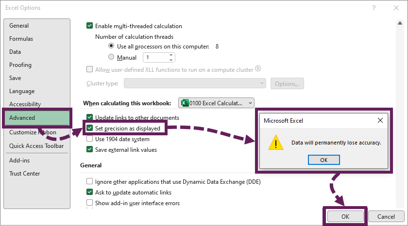
To apply Precision as Displayed:

• Click File > Options to open the Excel Options dialog box
• In the Advanced section, ensure set precision as displayed option is checked
• A warning message states that data will permanently lose accuracy; if you wish to proceed, click OK.
• Click OK to close the Excel options.

The formula will now calculate the correct result.

Wrap-up

Due to the nature of calculating floating point numbers, not all decimals can be perfectly expressed in binary. As a consequence, Excel can calculate the wrong result.

Excel applies the IEEE 754 standard to define how floating point numbers are calculated. Therefore Excel, like other applications, can sometimes calculate incorrect results. This is the complex world of mathematics and computing we all live in, rather than an issue with Excel.

Please beware of this issue. Make sure you check your results and, if necessary, apply the ROUND function to avoid the potential errors caused by calculations with floating point numbers.

Related Posts:

• Why are Excel formulas not calculating?
• Excel rounding vs Power Query rounding: WARNING They are different
• Why does Excel’s calculation mode keep changing?

---

What next?

Discover how you can automate your work with our Excel courses and tools.