GETPIVOTDATA vs CUBE functions

We’ve been able to create PivotTables in Excel since the mid-1990s. Ever since then, people have been asking how to extract data from PivotTables using formulas. As great as PivotTables are for analysis, they are not always the best for presentation, which is why extracting data using a formula is so useful. We currently have 3 options for this, standard cell linking, GETPIVOTDATA, and CUBE functions.

In this post, we will compare these three methods. This is not an in-depth look into any one approach but intended to highlight the differences so you can make the best decisions for your scenario.

Table of Contents

• Example data
• Standard formulas
• Extracting data from the PivotTable
• Changing data
• GETPIVOTDATA function
• Turn GETPIVOTDATA on/off
• Extracting data from the PivotTable
• Changing data
• Changing the GETPIVOTDATA function
• CUBE functions
• Creating a PivotTable with the Data Model
• Convert PivotTable to formulas
• Changing data
• Changing the CUBE functions
• Which is best?

Watch the video

Watch the video on YouTube.

Example data

All examples in this post use the same initial data set. This is available in the download file.

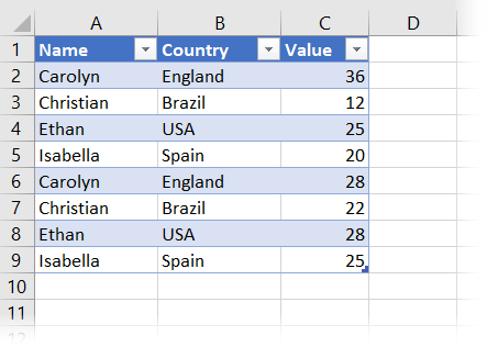
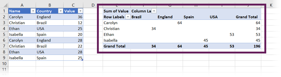
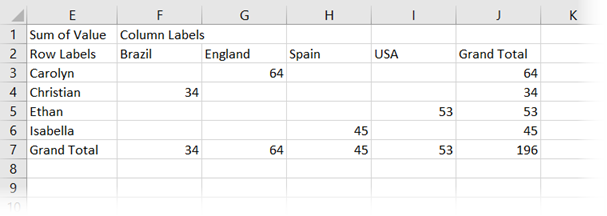
From that data set, I have created a PivotTable:

Please note that the PivotTable creation process requires an extra step when using CUBE functions. I will take you through this in the relevant section.

Standard formulas

PivotTables exist on Excel’s grid, with each cell on the grid having its own cell reference. Therefore, the simplest method of getting values from a PivotTable is to use standard cell references within a formula.

Extracting data from the PivotTable

As stated already, we can link any PivotTable item by using cell reference.

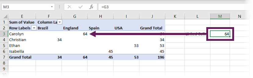
In the screenshot above, the formula in cell M3 is:

=G3

This formula extracts the value of 64 from the PivotTable, which is the Sum of Values for Carolyn in England.

Changing data

Now let’s change our source data. For this scenario, let’s suggest that Christian isn’t in Brazil, but in Finland. So, in our source, change cells B3 and B7 from Brazil to Finland, then click Data > Refresh All.

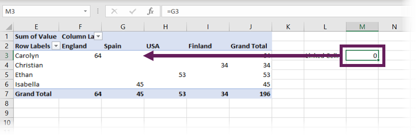
Look at the screenshot above. Our cell reference to G3 has been maintained. But the data point in that cell has changed, so we are now pointing to an empty cell. The Sum of Values for Carolyn in England is in cell F3, rather than G3.

The main lesson from cell linking is that cell references do not change when the position of the underlying data changes.
Note:
We could use a formula like INDEX / MATCH / MATCH to perform a 2-dimension lookup and ensure we extract the correct data for Carolyn in England. However, this defeats the benefit of using a PivotTable.

To avoid this issue, we can use one of the other extraction methods.

GETPIVOTDATA function

GETPIVOTDATA is the function most of us think about when needing to extract values from a PivotTable.

Turn GETPIVOTDATA on/off

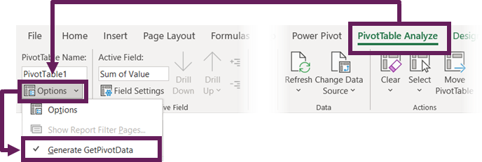
We can set Excel to automatically create the GETPIVOTDATA function when clicking on a PivotTable cell in a formula. To do this, select any cell in a PivotTable and click PivotTable Analyze > Options > Generate GetPivotData to ensure the option is turned on.

Now, each time we link to a PivotTable cell, the GETPIVOTDATA formula is created for us automatically.

Extracting data from the PivotTable

Let’s change our source data back to its original state and refresh the PivotTable. Next, let’s use GETPIVOTDATA to extract cell G3 from the PivotTable.

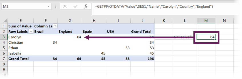
In the screenshot above, cell M3 contains the formula:

=GETPIVOTDATA("Value",$E$1,"Name","Carolyn","Country","England")

When clicking on cell G3, the GETPIVOTDATA function was automatically created for us. The individual elements breakdown as follows

• =GETPIVOTDATA – the name of the function
• “Value” – the name of the value field
• $E$1 – the top-left cell of the PivotTable
• “Name” – the name of the first Pivot Field
• “Carolyn” – the specific element from the first Pivot Field
• “Country” – the name of the second Pivot Field
• “England” – the specific element from the second Pivot Field

If there are more fields, we can continue to add these in pairs, just like “Country” and “England” have been above.

Changing data

Now let’s change our source data again from Brazil to Finland and click Data > Refresh All.

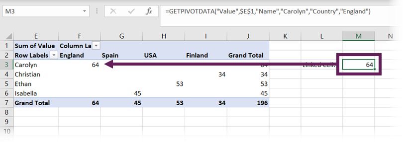
While the cell containing the data point has changed from G4 to F4, through GETPIVOTDATA, we are not linking to a cell. Instead, we are linking to the Sum of Value for Carolyn in England; therefore, the result returned is maintained.

Changing the GETPIVOTDATA function

We can make GETPIVOTDATA more flexible by using worksheet cells instead of hardcoded field names.

Linking Pivot Fields to cells

Let’s link an element from the Country field to a cell.

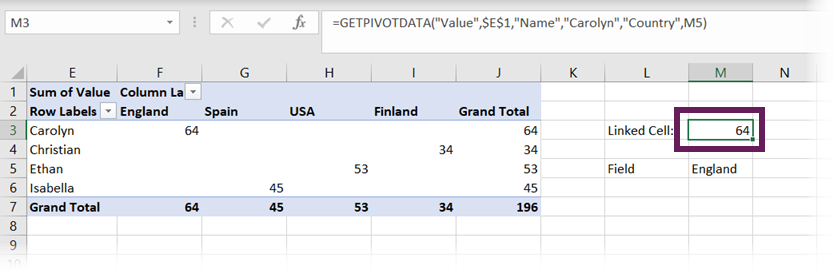
In the screenshot above, England has been entered into cell M5. GETPIVOTDATA has changed to the following:

=GETPIVOTDATA("Value",$E$1,"Name","Carolyn","Country",M5)

The formula references cell M5, which contains the field element.

We can change this to Spain, or USA, etc., and the GETPIVOTDATA will automatically recalculate.

Linking Data Fields to cells

So, what happens if we link the Data Field to a cell?

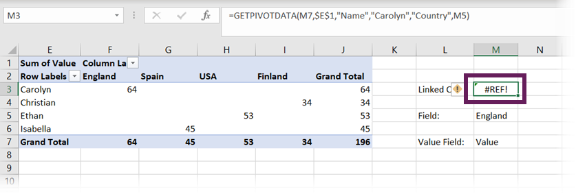
Oh! It doesn’t work. Cell M7 now contains the text Value, which is the name of the field in the value section of the PivotTable.

The formula in cell M3 is:

=GETPIVOTDATA(M7,$E$1,"Name","Carolyn","Country",M5)

But all is not lost. There is an odd workaround where we can add an empty text string at the start or end of the cell reference, and it will work.

If we change the formula in cell M3 to the following, it will work:

=GETPIVOTDATA(M7&"",$E$1,"Name","Carolyn","Country",M5)

Try it for yourself; it works!

CUBE functions

Let’s start this section by going back to our original data set.

A PivotTable can display information stored in either the Pivot Cache or the Data Model. These are the two methods of storing the data for the PivotTable. At creation, the Pivot Cache is used by default, but by clicking a single tick box, we can use the Data Model instead.

The Data Model is a more modern and efficient engine for handling data. Therefore, we should try to use the Data Model where we can.

The CUBE functions are a group of functions that can extract data from the Data Model. Since PivotTables and formulas can use the same source, the CUBE functions create the equivalent of extracting values from a PivotTable.

There are 7 CUBE functions, but for this post, we will only look at two: CUBEMEMBER and CUBEVALUE.

Creating a PivotTable with the Data Model

If we plan to use CUBE formulas, we must create a PivotTable in the right way.

Select a cell in the data set, then click Insert > PivotTable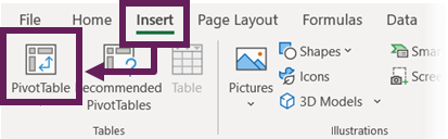

From the PivotTable from table or range window, select the Add this data to the Data Model option, then click OK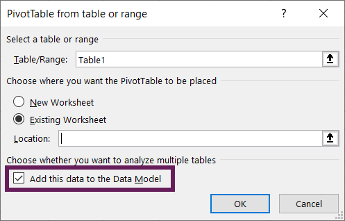

That’s it; there is only one additional click. The PivotTable will be created using the Data Model instead of the Pivot Cache.

We can add Pivot Fields and Value fields in the usual way.

Convert PivotTable to formulas

A PivotTable created from a Data Model can be converted into CUBE formulas.

Select a cell in the PivotTable, then click PivotTable Analyze > OLAP Tools > Convert to Formulas.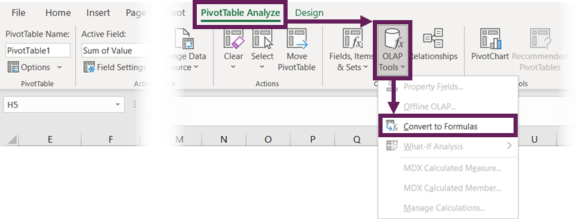

If your PivotTable has a field in the Filters section, the Convert to Formulas dialog will appear. We haven’t used the Filters section for this example, so this box will not appear. If it does for your scenario, select the option you want and click Convert.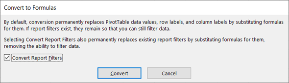

The PivotTable will now be converted into CUBE formulas. There is no PivotTable anymore!

We will cover how to manually change these formulas shortly.

Note:
While the formulas have been created by converting a PivotTable, if we learn the syntax required for CUBE formulas, we can write these ourselves just like other standard functions.

Changing data

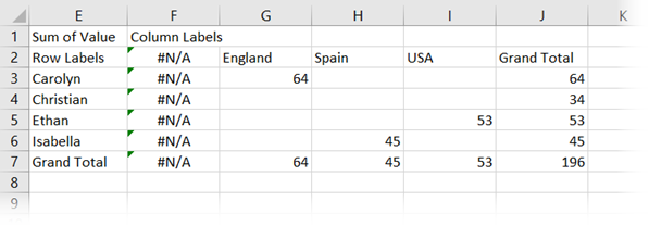
Now let’s change our source data again, from Brazil to Finland, then click Data > Refresh.

As we no longer have a PivotTable, it is the result of the formulas which are updated. Since there is no longer a field element called Brazil in our data set,  this is now displaying as #N/A.

Prove to yourself that this works. Change a number in the source data and click Data > Refresh All; the formula results will update.

Changing the CUBE functions

The transformation process to change the PivotTable to formulas uses two different functions: CUBEMEMBER and CUBEVALUE. We’ll take a look at each in turn.

CUBEMEMBER

The CUBEMEMBER formula is used for the dimensions/fields.

The formula in cell G2 is:

=CUBEMEMBER("ThisWorkbookDataModel","[Table1].[Country].&[England]")

This formula breakdowns as follows:

• =CUBEMEMBER – the name of the function
• “ThisWorkbookDataModel” – refers to the name of the data model being used. When using this methodology, the value will always be “ThisWorkbookDataModel”
• “[Table1].[Country].&[England]” – this is an MDX statement referring to the field element of England in the Country field from a table called Table1

The formula in cell E3 is:

=CUBEMEMBER("ThisWorkbookDataModel","[Table1].[Name].&[Carolyn]")

Notice that this is a very similar structure to cell G2 that we saw above. The difference is that we are referring to the field element of Carolyn in the Name field from a table called Table1.

The formula in cell E1 differs slightly:

=CUBEMEMBER("ThisWorkbookDataModel","[Measures].[Sum of Value]")

Cell E1 is not a field/dimension to filter by, but the calculation to be applied. Therefore, it has a slightly different format.

“[Measures].[Sum of Value]” – This is the syntax for referring to an implicit measure created in a PivotTable. The first item in the square brackets will always be Measures, with the name of the calculation in the second set of square brackets.

For CUBE functions, anything in double-quotes is a text value and can be linked to a cell, or concatenated with other text strings.

CUBEVALUE

The CUBEVALUE formula retrieves values from the Data Model based on the filter context created by the CUBEMEMBER functions it is linked to.

The formula in cell G3 is:

=CUBEVALUE("ThisWorkbookDataModel",$E$1,$E3,G$2)

This formula breakdowns as follows:

• =CUBEVALUE – the name of the function
• “ThisWorkbookDataModel” – refers to the name of the data model being used
• $E$1,$E3,G$2 – these are all cell links to the relevant CUBEMEMBER functions above

The CUBEMEMBER function provides the fields to use, and the CUBEVALUE retrieves the value for that filter context.
Note:
It is possible to change the reference to the calculation to be performed, for example, changing from [Measure].[Sum of Value] to [Measure].[Max of Value]. However, there is a quirk to be aware of.

Unless writing explicit measures using DAX in PowerPivot, all implicit calculations must be created within a PivotTable before referring to it in a formula. If we wanted to use [Measures].[Max of Value] we would first need to create a PivotTable, with that calculation included.

Once created, that implicit measure/calculation is available for the CUBE functions to use.

Which is best?

Which is the best option to use? Unfortunately,…. it depends.

The best is relative to your scenario. Since the Data Model is more efficient at handling data than the Pivot Cache, that would always be my preferred method. Plus, there is the added benefit that this is a stepping stone to using the Power Pivot tool in Excel.

This was an introduction to the differences between GETPIVOTDATA and CUBE functions for extracting data from a PivotTable. But, please don’t end your journey here, there is so much more to learn:

• Tips & Tricks for Writing CUBEVALUE Formulas – Excel Campus: https://www.excelcampus.com/cubevalue-formulas/
• Cube Formulas – The best Excel formulas you’re not using – Macrodinary: https://macrordinary.ca/2020/08/19/cube-formulas-the-best-excel-formulas-youre-not-using/
• An intro to Cube functions for PowerPivot – BI Gorilla: https://gorilla.bi/excel/cube-functions/
• How to use PivotTable – GetPivotData – Contextures: https://www.contextures.com/xlpivot06.html
• Excel GETPIVOTDATA function: Excel Jet: https://exceljet.net/excel-functions/excel-getpivotdata-function

---

What next?

Discover how you can automate your work with our Excel courses and tools.