How to filter by a list in Power Query (4 methods)

Filtering is a common task in Power Query. Usually, we filter by a single value, or maybe a small number of known values. These filter values are hardcoded into the underlying M code. Therefore, to change the filter, we have to edit the query. But what if we don’t know which items we want to filter by, or how many items there are? Well, that’s what we’ll find out in this post, by looking at how to filter by a list in Power Query.

Table of Contents

• Example
• Understand filtering in Power Query
• Filter by a list
• List.Contains syntax & arguments
• Convert the FilterList table into a list
• Amend the Table.SelectRows function
• Testing the solution
• Do we have to convert FilterList to a list?
• Filter to exclude items
• Merge – alternative faster approach
• Merge vs List.Contains – which is faster?
• Filter columns by a list
• Dynamic filtering
• Conclusion

Watch the video

Watch the video on YouTube

Example

The example data we are working with in this post is as follows:

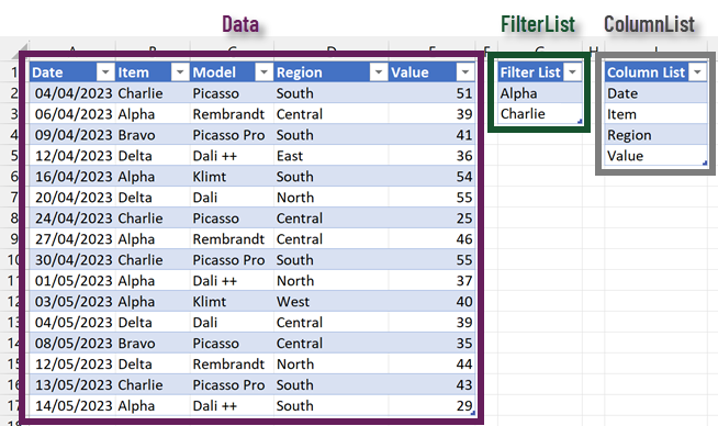
The examples all use data in Excel Tables, but could be from any sources. The Table names are:

• Data: The data we wish to filter
• FilterList: The values we want to filter the Item column of the Data table by
• ColumnFilter: Used in the example below to demonstrate how to filter the columns in the output.

In the example file, all three tables are loaded into Power Query.

Understand filtering in Power Query

Let’s start by filtering with the user interface to understand the M code syntax.

Click on the filter button at the top of the Item and select Alpha and Charlie.

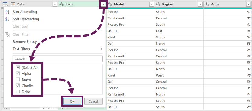
The M code for this step is:

= Table.SelectRows(#"Changed Type", each ([Item] = "Alpha" or [Item] = "Charlie"))

Let’s break this formula down

• Table.SelectRow: The formula for selecting rows in a Table
• #”Changed Type”: The name of the table to filter (usually the name of the previous step)
• each: A keyword to indicate the following code section is applied on a row-by-row basis
• ([Item] = “Alpha” or [Item] = “Charlie”): A logical test to check if the value in the Item column equals Alpha or Charlie

The logical test is the element we need to change for more advanced filtering.

If we amended the formula as follows, all the rows are returned.

= Table.SelectRows(#"Changed Type", each true)

Or, if the formula were as follows, none of the rows are returned:

= Table.SelectRows(#"Changed Type", each false)

Therefore, to filter based on a list, we need a formula that returns True or False for each row in the table. True items are retained, false items are excluded.

Filter by a list

To filter by a list, we use the List.Contains function.

List.Contains syntax & arguments

List.Contains checks if a value exists inside a list. The syntax and arguments for List.Contains are as follows:

Syntax:

List.Contains(list as list, value as any, optional equationCriteria as any) as logical

Arguments:

• list: the list of values
• value: the value to check if it exists in the list
• equationCriteria: determines how values are compared (e.g., whether to ignore case)

The equationCriteria argument can become quite complex. This is outside the scope of this post. To find out more, check this out: https://blog.crossjoin.co.uk/2017/01/22/the-list-m-functions-and-the-equationcriteria-argument/

Result: The output of List.Contains is a logical value (i.e., True or False)

More info: Find more information on List.Contains here: https://learn.microsoft.com/en-us/powerquery-m/list-contains

Convert the FilterList table into a list

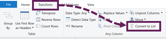
The FilterList query is currently a Table; we need to convert this into a list.

Select the FilterList query, then click Transform > Convert to List

Amend the Table.SelectRows function

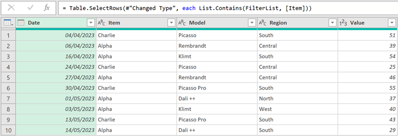
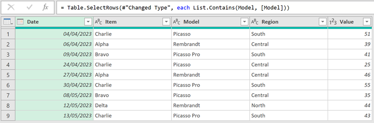
Select the Data query, and find the Filtered Rows step we created earlier. Amend the formula as follows:

= Table.SelectRows(#"Changed Type", each List.Contains(FilterList, [Item]))

• FilterList: The name of the list query
• [Item]: The name of the column to filter. The each keyword ensures this comparison occurs row by row

The preview window displays the result:

Currently, case is considered in the filter; “alpha” and “Alpha” are considered different values. To ignore the case, we would add an equationCriteria argument to the formula as follows:

= Table.SelectRows(#"Changed Type", each List.Contains(FilterList, [Item], Comparer.OrdinalIgnoreCase))

Testing the solution

Close and load the queries and return to Excel.

Change the values in the FilterList table, then click Data > Refresh All.

Ta Dah! The query refreshes to show only the items in the list.

Do we have to convert FilterList to a list?

We may have other uses for the FilterList query; therefore, we may not want to convert it to a list.

In that scenario, we could create the list inside the List.Contains function; this avoids changing the FilterList table query.

= Table.SelectRows(#"Changed Type", each List.Contains(FilterList[Filter List], [Item]))

• FilterList: the name of the query
• [Filter List]: the name of the column to convert to a list

Filter to exclude items

Another common scenario is to filter out the items from the table. To achieve this, we add the word not to the function; this flips the True and False results around.

 Table.SelectRows(#"Changed Type", each not List.Contains(FilterList, [Item]))

Merge – alternative faster approach

If we have a reasonably simple filter scenario, but a lot of data, we can use the merge transformation as an alternative.

In the merge transformation, assuming we have the Data table first, and the FilterList table second, we use a Right Outer join to return only the items in the filter table. See the example below:

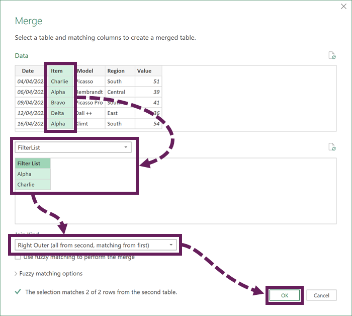
Once the merge is returned, we can delete the merged column as it is not required. This creates the same effect as filtering by a list.

Merge vs List.Contains – which is faster?

I tested the Merge and List.Contains methods for speed; the result is surprising.

Test #1: 100,000 rows of 8 unique values, which is filtered by 2 values:

• List.Contains: 18.2 seconds
• Merge with right-outer join: 1.6 seconds

Test #2: 100,000 rows of 8 unique values, which is filtered by 4 values:

• List.Contains: 26.3 seconds
• Merge with right-outer join: 1.7 seconds

This shows that merge is significantly faster.

Filter columns by a list

OK, we now understand how all this works. Time to take it to the next level. Let’s filter the column names to return only the columns we want.

Convert the ColumnList query to a list by selecting it, then clicking Transform > Convert to List.

In the Data query, select some columns, then click Home > Remove Columns (drop down) > Remove Other Columns.

The M code for the step looks like this:

= Table.SelectColumns(#"Filtered Rows",{"Date", "Item", "Model"})

The M code lists the columns we retained. To make this dynamic, we just need to replace the list of hard-coded values with our ColumnList query.

= Table.SelectColumns(#"Filtered Rows",ColumnList)

This also places the columns in the same order as the list.

Note: I recommend performing this step at the end, because if other steps reference columns that have been removed, it will cause an error.

Dynamic filtering

OK, now for our final example. Let’s suggest we want to return only the rows for the top 3 Models. However, over time, as our data changes, so will the top 3 models. Our list to filter by is not fixed. Therefore, we need to make this completely dynamic.

Select the Model column, then click Transform > Group By.

In the Group By dialog box, enter the following:

• New Column Name: Total
• Operation: Sum
• Column: Value

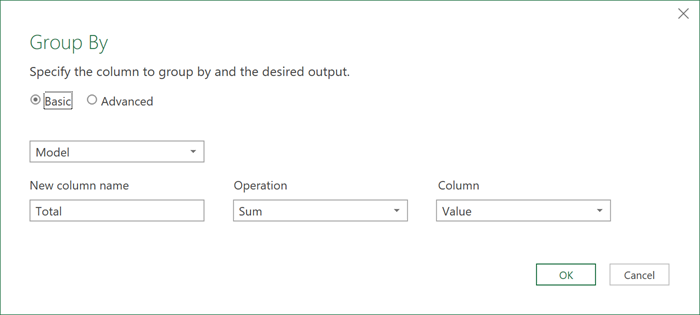
Click OK to close the Group By dialog box and display the summarized values.

To sort the values, select the Total column, then click Home > Z-A.

Next, we need to keep only the top 3 rows. Click Home > Keep Rows (drop down) > Keep Top Rows

In the Keep Top Rows dialog box, enter 3 into the number of rows field, then click OK.

Select the Model column, then click Transform > Convert to List.

Click on the fx icon in the formula bar. Enter the following formula:

= Table.SelectRows(#"Changed Type", each List.Contains(Model, [Model]))

• #”Changed Type”: The name of the step where the full data was last available
• Model: The name of the previous step, which created the list
• [Model]: The column name to filter by

The preview window displays the following:

We now have a dynamic filter list. When the source data changes, the list for the top 3 models is re-calculated. That dynamic list is used to filter the table.

Conclusion

In this post, we have seen how to filter by a list in Power Query. This was achieved using the List.Contains function which returns a True or False result for each row in a table. We also used the right-outer join of the merge transformation to create a filtering effect; this was significantly faster than List.Contains.

Finally, we explored how to filter column names and how to create a dynamic filter to display results for the top n elements.

Related Posts

• Power Query: Lookup value in another table with merge
• How to get data into Power Query – 5 common data sources
• Common Power Query errors & how to fix them

---

What next?

Discover how you can automate your work with our Excel courses and tools.