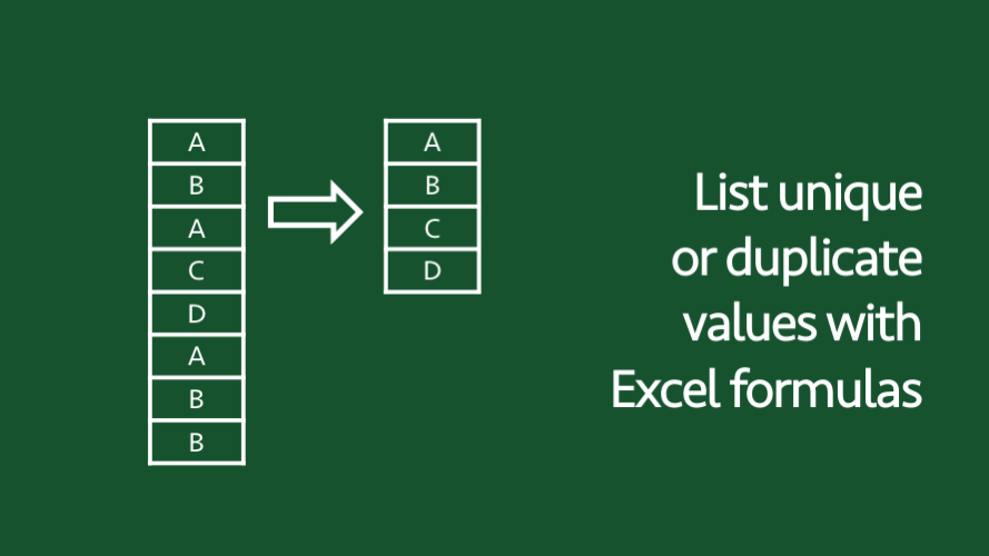
The Excel team recently announced new dynamic array formulas, which can create unique lists, sort and filter with a simple formula. These new formulas are being rolled out to Office 365 subscribers over the next few months. However, not everybody has the subscription and will upgrade when it is sensible for their business, often combining it with a hardware refresh. Therefore, it could be 6 or more years before enough users have the new functionality to use it safely and ensure compatibility. So how can we list duplicate values, or unique values in Excel using traditional Excel methods? We will cover that in this post.
COUNTIF is an untapped powerhouse for most Excel users. Counting cells which meet specific criteria may not seem particularly useful, but when combined with other functions, and boolean (true/false) logic, it creates new capabilities you never thought possible.
This post looks at one aspect of this and considers how to use the COUNTIF function to create and compare lists to check for duplicate or unique values. We’ll start with some basic scenarios and slowly layer on the complexity until we achieve some advanced formula magic.
Comparing two unique lists
The COUNTIF function can be used to compare two lists and return the number of items within both lists.
Let’s look at an example. In the screenshot below there is a list of students from St John’s school (Cells A2 – A7) and a list of students who attended a specific exam (Cells B2-B6). We have been asked to identify the number of individuals who are on both lists (i.e., how many from St John’s school attended the exam).
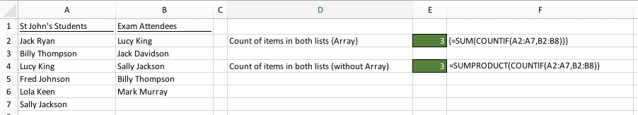
The formula in Cell E2 is:
{=SUM(COUNTIF(A2:A7,B2:B6))}
Usually, COUNTIF will count the number of items from a list which meet a single criteria. In this case, we have not provided a single criteria, but have used a range of cells. As we have not used any logic operators, such as greater than ( > ), Excel by default, applies equals ( = ) as it’s logic operator. This formula will therefore, compare each cell in the Range B2 – B6 to identify if it is equal to any cells in the Range A2 – A7.
In this example, there are multiple calculations all occurring within the same formula. Calculation 1 compares Cell B2 to Cells A2:A7, calculation 2 compares Cell B3 to Cells A2:A7, etc etc. In total there are 5 separate results all calculated at the same time; this type of formula is known as an array formula.
The COUNTIF function will calculate down as follows:
{=SUM({1;0;1;1;0})}
Notice how all 5 results are shown, each separated by a semi-colon. By wrapping this within the SUM function it will add the list of 1’s and 0’s, which is the number of items which appear on both lists.
As this is an array formula do not type the curly bracket at the start or end of the formula, Excel will include these itself when you press Ctrl + Shift + Enter to enter the formula into the cell or formula bar.
If we wanted to avoid pressing the Ctrl + Shift + Enter, we could use the SUMPRODUCT function, rather than the SUM function. The formula in Cell E4 is:
=SUMPRODUCT(COUNTIF(A2:A7,B2:B6))
SUMPRODUCT is a special function which can handle arrays without the need for Ctrl + Shift + Enter.
Usually, SUMPRODUCT is used to multiply cells or numbers together then add the results of the multiplications. In the way we are using it, there is no multiplication occurring within the SUMPRODUCT function, so it will just sum the result.
Comparing lists with duplicates
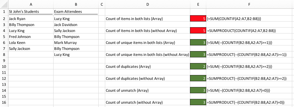
In the example above, both lists are unique, but what if one of the lists contains duplicates? In this scenario, the result of the formula would be incorrect. I have expanded the example to include duplicates for two Exam Attendees (see screenshot below), Lucy King and Billy Thompson now appear twice in column B. The result of the previous calculation is shown in cells E2 and E4. The result of which is incorrectly calculated as 5. The result has increased by 2 due to the duplicate values.
When working with unique data it does not matter which list is used in each argument of the COUNTIF function. However, when there are duplicates the first range in the function must be the range containing the duplicates and the second range containing the unique values. Please note this change within the examples for the remainder of this post.
Count unique items
The formula in Cell E6 is:
{=SUM(--(COUNTIF(B2:B8,A2:A7)>=1))}
This formula is an extension of the example in the section above, but it adds some additional complexity. Let’s take some time to understand how it works.
A logic test has been added to the formula so that only items where the count is >=1 (i.e., unique values) are included.
{=SUM(--(COUNTIF(B2:B8,A2:A7)>=1))}
This logic statement will calculate to TRUE or FALSE.
{=SUM(--({FALSE;TRUE;TRUE;FALSE;FALSE;TRUE}))}
It is not possible to use SUM on TRUE or FALSE values. These will need to be converted into values of 1 for TRUE or 0 for FALSE to enable the SUM function to work. There are two options for this:
- Multiply TRUE/FALSE values by 1
- Multiply TRUE/FALSE values by – – (minus, minus).
On our example, I have opted to use the double minus method. Now the formula has calculates down as follows:
{=SUM({0;1;1;0;0;1})}
The SUM function will return the value of 3, which is correct.
If we wanted to avoid Ctrl + Shift + Enter, SUMPRODUCT is an option, as shown in Cell E8:
=SUMPRODUCT(--(COUNTIF(B2:B8,A2:A7)>=1))
Count duplicates
By applying the same formulas, but changing the logic threshold we can calculate the number of duplicate values.
The formula in Cell E10 is:
{=SUM(--(COUNTIF(B2:B8,A2:A7)>=2))}
As the logic statement requires values greater than or equal to 2, it will only count the duplicates.
Again we can use SUMPRODUCT to avoid pressing Ctrl + Shift + Enter, as shown in Cell E12:
=SUMPRODUCT(--(COUNTIF(B2:B8,A2:A7)>=2))
Count unmatched items
The final measure of interest may be the number of items not matching either list. For this, the logic statement changes again to show only the items where the count is equal to zero.
The formula in Cell E14 is:
={SUM(--(COUNTIF(B2:B8,A2:A7)=0))}
The non-Ctrl + Shift + Enter version in Cell E16 is:
=SUMPRODUCT(--(COUNTIF(B2:B8,A2:A7)=0))
Extract a list of unique values
Using this concept of comparing two lists with COUNTIF, we can not only count unique values, but also extract a list of unique values.
The example data has now changed. Column A contains a list of students who attended an exam, but it contains duplicates. We will use this data to create a unique list of value, as shown in Column B.
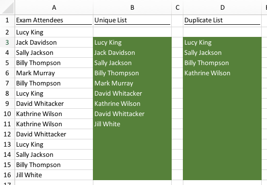
The formula in Cell B3 is:
{=IFERROR(INDEX(A$2:A$16,MATCH(0,COUNTIF(B2:B$2,A$2:A$16),0)),"")}
This is an array formula which requires Ctrl + Shift + Enter.
This formula uses what we have already learned about COUNTIF and expands it even further. Let’s explore this in more detail.
Understanding the formula
{=IFERROR(INDEX(A$2:A$16,MATCH(0,COUNTIF(B2:B$2,A$2:A$16),0)),"")}
Notice how the COUNTIF function includes a relative and an absolute cell reference to the row numbers within the first argument (B2:B$2), this ensures that when the function copies down the range of cell increases in size.
For this first cell there is nothing in our list of unique values (as the unique list is currently just the blank value in Cell B2), therefore the COUNTIF returns zeros for every result.
{=IFERROR(INDEX(A$2:A$16,MATCH(0,{0;0;0;0;0;0;0;0;0;0;0;0;0;0;0},0)),"")}
Next, we’ll look at the MATCH function.
{=IFERROR(INDEX(A$2:A$16,MATCH(0,{0;0;0;0;0;0;0;0;0;0;0;0;0;0;0},0)),"")}
This function returns the position of the first 0 using the exact match method. The result of the MATCH function is 1 because the first 0 is in the first position.
{=IFERROR(INDEX(A$2:A$16,1),"")}
Next, the INDEX function will find the cell in the Range A2 – A16 which has a position of 1 (i.e., the first cell). This calculates down as follows:
{=IFERROR("Lucy King","")}
When using this formula, we do not have to know how many unique values there are as the IFERROR function ensures a blank is returned once the bottom of the unique list is reached.
Copy down the formula
Drag the formula in Cell B3 down to provide enough rows for the current data and any future growth.
It is difficult to appreciate this formula by looking only at the first result, therefore to get a better understanding of how this formula really works look at Cell B4.
{=IFERROR(INDEX(A$2:A$16,MATCH(0,COUNTIF(B$2:B3,A$2:A$16),0)),"")}
COUNTIF will now down calculate as follows:
{=IFERROR(INDEX(A$2:A$16,MATCH(0,{1;0;0;0;0;0;1;0;0;0;0;1;0;0;0},0)),"")}
There are now 1’s within the result. These occur each time the values in Cells B2 – B3 appear in Cells A2 – A16. When the MATCH function looks for 0’s it will now return the 2nd item in the list (which is the next unique item).
For the next example, check out Cell B6:
{=IFERROR(INDEX(A$2:A$16,MATCH(0,{1;1;1;0;0;0;1;0;0;0;0;1;1;0;0},0)),"")}
As more items are now included within the unique list (which has now grown to Cells B2 – B5) more 1’s will appear. The fourth item in the list is the first zero, so that value is returned.
As the formula copies down further there will be less 0’s remaining.
When there are no 0’s remaining (i.e., the list contains all the unique values) the MATCH function will return errors. These errors are captured by the IFERROR statement and turned into blank cells with two quotation marks (“”).
If you wish to avoid Ctrl + Shift + Enter, we cannot use SUMPRODUCT as before. Instead, we can use the INDEX function to process the array. The change required is highlighted below.
=IFERROR(INDEX(A$2:A$16,MATCH(0,INDEX(COUNTIF(B2:B$2,A$2:A$16),),0)),"")
List duplicate values
Having looked at extracting a list of unique values, we now move on to consider extracting a list of duplicate values.
The formula in Cell D3 is so long that it is included on two lines below, but you can have it on a single line within Excel.
=IFERROR(INDEX(A$2:A$16,MATCH(1,
((COUNTIF(D2:D$2,A$2:A$16)=0)*(COUNTIF(A$2:A$16,A$2:A$16)>=2)),0)),"")
The differences to the unique formula in the section above are highlighted below:
{=IFERROR(INDEX(A$2:A$16,MATCH(1,
((COUNTIF(D2:D$2,A$2:A$16)=0)*(COUNTIF(A$2:A$16,A$2:A$16)>=2)),0)),"")}
The first COUNTIF function has changed to include a logic test for where the value equals 0. We know that 0 appears where the item does not already appear in the list. If it equals 0 the result will be TRUE, otherwise it will be FALSE.
The second COUNTIF function is comparing the source list to itself to count the number of instances of each value. Where the count is greater than or equal to 2 (i.e., it is a duplicate value) TRUE will be returned, otherwise it will return FALSE.
As we now have two lists of TRUE/FALSE we can multiply these together. Where there are two TRUE values (i.e., the value appears more than once in the master list and it does not already appear in our list of duplicates). the multiplication returns 1, all other values will contain a FALSE value, so will multiply to 0.
We change the MATCH function to find 1, rather than 0.
Drag this formula down, and we have created a list of duplicate values.
Once again, if you wish to avoid Ctrl + Shift + Enter, use the INDEX function to process the array. The change required is highlighted below.
=IFERROR(INDEX(A$2:A$16,MATCH(1,
INDEX(((COUNTIF(D2:D$2,A$2:A$16)=0)*(COUNTIF(A$2:A$16,A$2:A$16)>=2)),)
,0)),"")
Why use a complicated formula?
But there are plenty of other options for creating unique lists and identifying duplicates:
- Pivot Table
- Power Query
- Remove Duplicates from the Data Ribbon
Each of these options is easier to understand than the complex formulas we have created, so why bother them? Wouldn’t it be easier to use one of those other methods? Yes and No.
Those options all require either a macro or user interaction to work. For Pivot Tables and Power Query the user must “Refresh” the data. For Remove Duplicates, the user must manually remove the duplicates each time a change occurs.
A formula has one significant advantage; it can be completely dynamic and automatically update when the data changes. If the source data is either an Excel Table or a Dynamic Named Range the list of unique or duplicates can be updated even when new data is added is added to the source data. In my opinion, this makes it a much more usable solution.
Until we get the new dynamic array formulas are rolled out and well established, the methods above are probably these option available.
Conclusion
As we have seen, the simple COUNTIF function is significantly more powerful than most Excel users realize. By using a range as the criteria we were able to create an array formula which holds multiple calculations within a single cell. Then, when combined with INDEX and MATCH it is possible to list unique or list duplicate values.
Understanding how Excel handles TRUE/FALSE is a crucial part of creating advanced formulas within Excel.
Related Posts:
Discover how you can automate your work with our Excel courses and tools.
The Excel Academy

Make working late a thing of the past.
The Excel Academy is Excel training for professionals who want to save time.
Thank you for the very clear explanation. I appreciate your time and effort!